Variational Inference using Implicit Models, Part I: Bayesian Logistic Regression
This post is part of a series of tutorials on using implicit models for variational inference. Here's a table of contents so far:
- ➡️️Part I (you are here): Inference of single, global variable (Bayesian logistic regression)
- Part II: Amortised Inference via the Prior-Contrastive Method (Explaining Away Demo)
- Part III: Amortised Inference via a Joint-Contrastive Method (ALI, BiGAN)
- Part IV: Using Denoisers instead of Discriminators
I've written a lot here about generative modeling, and in particular about the theory of GANs. GANs provide a new set of tools for dealing with a nasty class of generative distributions. I'm going to follow Shakir and Balaji's terminology and call them implicit generative models: probabilistic models which
- we can sample from easily, and
- we can take the derivative of samples with respect to parameters
Such probabilistic models are useful in general, not only for generative modelling. Here, I'm going to show a simple example of how to use them for approximate inference. This is part one of what I hope will be a series of posts, starting with the simplest setup. Here's a table of contents for the whole series:
Approximate inference of a single global variable
To simplify things, I'm only going to talk about is approximate inference of a single, global hidden variable (rather than one hidden variable per observation such as for example variational autoencoders). A simple example I'm going to use is Bayesian logistic regression, whose graphical model looks like this:
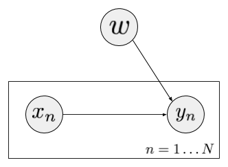
Here, we have a number of observed input values $x_n$ and a global parameter $w$. For each input we also observe a binary output label $y_n$. Our model specifies that this label depends on the corresponding observation $x_n$ and the global parameter $w$ in the following way:
$$
\mathbb{P}(y_n=1 \vert x_n, w) = \Phi(w^{T}x_n),
$$
where $\Phi$ denotes the logistic sigmoid.
In this model I would like to perform Bayesian inference of $w$ which involves calculating $p(w\vert \mathcal{D})$, where $\mathcal{D} = {(x_n y_n), n=1\ldots N}$ denotes the observations. The problem is, once you have many observations, this posterior is intractable to compute exactly. We would like to approximate it with a simpler distribution.
Variational Inference and Density Ratios
One common way to perform approximate inference is by variational methods. Here, one aims to minimise the KL (or other) divergence between $q$ and the real posterior $p$. This, unfortunately, is only possible exactly if $q$ is simple enough and compatible with the prior $p$. This usually severely limits the power and expressivity of approximate posteriors to boring, often factorised, Gaussians and other exponential families. We would like to use something more powerful, and in this post, I want to use an implicit probabilistic model $q$ which I can sample from. Here is how one can do this:
\begin{align}
\operatorname{KL}[q(w),p(w\vert \mathcal{D})] &= \mathbb{E}_{w\sim q} \log \frac {q(w)}{p(w\vert \mathcal{D})}\\
&= \mathbb{E}_{w\sim q} \log \frac {q(w)}{p(w)} - \mathbb{E}_{w\sim q} \log p(\mathcal{D}\vert w) + \log p(\mathcal{D})
\end{align}
The final term is the marginal likelihood, wihch doesn't depend on the parameter so it can be ignored when optimising for $q$. In this expression, we have the probability ratio between the prior $p(w)$ and the approximate posterior $q(w)$. We know how to approximately learn probability ratios, for example by using logistic regression. This suggests a simple, adversarial-type iterative training algorithm with the following losses:
\begin{align}
\mathcal{L}(D; G) &= \mathbb{E}_{w\sim q} \log D(w) + \mathbb{E}_{w\sim p} \log (1-D(w))\\
\mathcal{L}(G; D) &= \mathbb{E}_{w\sim q} \log \frac{D(w)}{1 - D(w)} - \mathbb{E}_{w\sim q} \log p(\mathcal{D}\vert w)\\
&= \mathbb{E}_{z} \log \frac{D(G(z))}{1 - D(G(z))} - \mathbb{E}_{z} \log p(\mathcal{D} \vert G(z))
\end{align}
We iterate two steps: we train the discriminator by minimising $\mathcal{L}(D; G)$ keeping $G$ fixed, and then we fix $D$ and take a gradient step to minimise $\mathcal{L}(G; D)$.
Does this work?
I coded this simple toy problem of Bayesian logistic regression up in theano/numpy. Here is the link to ipython notebook - it's pretty poorly organised, but I hope it's readable enough and serves as proof of concept. I conditioned on just three observations, manually chosen, and two dimensional weight vector $w$. This is what the final results look like:
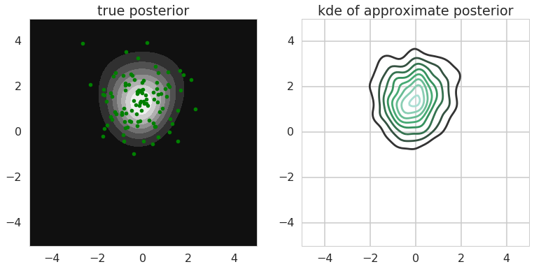
The left-hand plot shows a heatmap of the true log posterior (up to normalisation constant) and 100 samples from the implicit probabilistic model $q$ overlaid. On the right-hand plot I show the kernel density estimate of $q$ from $n=20000$ samples. We can see that the posterior was recovered nicely by $q$, both its mean and it's rough shape. I used simple 3-layer MLP with 10-20 hidden units on each layer with relu activations to get this, so the model is not super-powerful, nor did I spend a lot of time tweaking the optimization, so it is probably possible to get even better results.
Let's look at what the discriminator converged to (yes, they all actually converge, as this is a very simple toy problem):
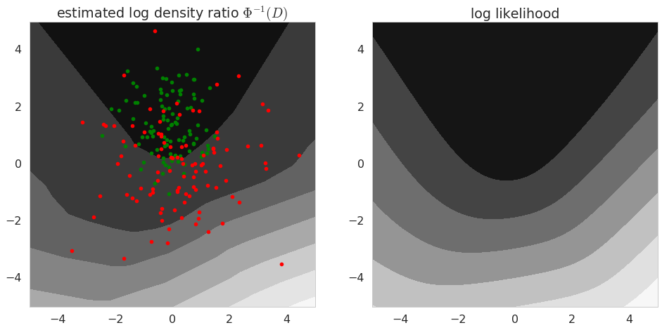
The left-hand plot shows the contours of our estimate of the log-density ratio $\log\frac{q}{p}$ extracted from the discriminator by taking the inverse sigmoid $\Phi^{-1}$. As $q$ converges to the real posterior, this log density ratio should converge to the log likelihood (shown on the right), up to a constant. The constant difference between the left-hand and right-hand plots is an estimate of the log marginal likelihood. The left-hand plot also shows samples from the prior in red and samples from the approximate posterior $q$ in green.
Note that the discriminator converges to the log-likelihood, without seeing any data itself. The discriminator is only trained via the prior and $q$, only $q$ has a data-dependent term in its loss function.
A few relevant papers
This post is not rocket science, and it was only meant to show how the GAN idea can be used more generally than sampling pretty pictures. Things like this have of course been used in many papers, here I'm just highlighting a few.
For example, it is very similar to what adversarial autoencoders try to do. There, adversarial training is used in an amortized inference setup: instead of one global variable we have hidden variables sampled for each observation. In adversarial autoencoders the adversarial loss is introduced between the prior and the average variational posterior $\tilde{q}(z) = \mathbb{E}_{x\sim p}q(z\vert x)$. I leave it as homework for you to figure out whether one can do something smarter, or more principled.
Another relevant paper is the one on Adversarial Message Passing by Theo Karaletsos. Here, the key observation is that the simple method outlined here may not scale very well to high-dimensional joint distributions, and in such cases it may be more useful to restrict the adversarial training to local computations in a message passing scheme on a factor graph.
Similar ideas are also discussed in (Donahue et al, 2016, BiGANs) and (Dumoulin et al, 2016, Adversarially Learned Inference). As Dustin pointed out in his comment below, the variational programs in (Ranganath et al. 2016, Operator Variational Inference) can also be thought of as implicit probabilistic models, while Stein variational gradient descent method of (Liu and Wang, 2016) directly optimises a set of samples to perform variational inference.
It is quite possible I'm missing references to other relevant papers, too, so please feel free to point these out in the comments.
Criticism
I can see the following criticisms of the simple method outlined here:
- This method behaves too much like noise-contrastive divergence, in that the prior $p(w)$ is probably much wider compared to $q(w)$. The logistic-regression-based density ratio estimation method works best if the two distributions are quite similar to each other. If they aren't we probably need a large number of samples from the prior to explore the interesting parts of the prior $p$. One could think about using the an analytically tractable variational baseline as the reference distribution instead of the prior, and the performance would probably be better in general.
- The method does not exploit any knowledge we might have about the prior $p(w)$. It is usually well-behaved and available in an analytical form. If the prior is a nice Gaussian, why wouldn't we just plug in the simple quadratic form to express its log-density, why do we have to learn it with an overparametrised neural network? This sounds wasteful. I'll address this in a follow-up post and suggest an alternative algorithm to fix this.
- Are neural networks really needed here? This echoes my criticism of adversarial autoencoders. Adversarial learning is really useful when faced with the 'complicated' manifold-like distributions such as the distribution of natural images. GANs work well at least in part because they use convolutional neural networks which provides a very strong and useful inductive bias as to what these algorithms can learn to do. When applying adversarial training to the problem of variational inference, we are now working with very different kinds of distributions. They can be high-dimensional but in many cases the prior is a simple Gaussian, or a structured graphical model.
Summary
GAN style algorithms have been developed mainly for generative modelling to model distributions of observed data. They can, too, be applied to approximate inference, where one uses them to model distributions over latent variables. What I showed here is perhaps the simplest formulation one could come up with to do this, but it is not hard - at least in theory - to generalise this furter to, say, amortized approximate inference. I'll try and follow up with a few posts on these extensions.