Variational Inference using Implicit Models Part IV: Denoisers instead of Discriminators
This post is part of a series of tutorials on how one can use implicit models for variational inference. Here's a table of contents so far:
- Part I: Inference of single, global variable (Bayesian logistic regression)
- Part II: Amortised Inference via the Prior-Contrastive Method (Explaining Away Demo)
- Part III: Amortised Inference via a Joint-Contrastive Method (ALI, BiGAN)
- ➡️️Part IV (you are here): Using Denoisers instead of Discriminators
That's right, I went full George Lucas and skipped Part III because (a) it was your homework assignment to write that for me and (b) following up Part II with Part III is relatively boring and predictable and the stuff in this post is way more interesting! This is the rogue one. This is about replacing density ratio estimation (a.k.a. the discriminator) with denoising as the main tool to deal with implicit models.
Summary of this note
- I explain how denoisers can be used to estimate the gradients of log-densities, which in turn can be used in a variational algorithm
- I derive simple variational inference algorithms based on denoisers for Bayesian logistic regression and for amortised VI
- I discuss related work and why the reconstruction error should not be used as a substitute for the energy
- finally, I discuss the toy experiments I did in the associated iPython notebook
Rationale
The key difficulty in using implicit models is that their log density (also known as energy) is unknown. My way to understand GANs is that they use logistic regression to estimate the log density relative to some other distribution. In generative modelling we measure the log density ratio to the target data distribution, in VI to the prior, or between joint distributions. Crucually, training the discriminator only requires samples from the implicit model (and from the contrast distribution) which makes this possible.
Denoising provides another mechanism to learn about the log density of a distribution only requiring samples. Instead of learning a log density ratio, the denoiser function learns the gradient of the log density, also known as the score or score function in statistics. We can then use these gradient estimates with the chain rule to devise an algorithm that maximises or minimises functionals of the log density, such as entropy, mutual information or KL-divergence.
Derivation
Let's take an implicit probability distribution $q(x; \phi)$ over a $d$-dimensional Euclidean space $\mathbb{R}^d$. Let's say we sample from $q$ by squashing normal random vectors $z$ through a nonlinearity G, so that $z\sim \mathcal{N}(0,I), x=G(z; \phi)$ is the same as writing $x\sim q(x; \psi)$.
Now consider training a denoising function $F:\mathbb{R^d\rightarrow R^d}$ so as to minimise the average mean-squared reconstruction error, that is
$$
F^{*} = \operatorname{argmin}_F \mathbb{E}_{x\sim q(x; \phi)} \mathbb{E}_{\epsilon \sim \mathcal{N}(0, \sigma^2I)}|F(x+\epsilon) - x|^2
$$
In the formula above, $\epsilon$ is additive isotropic Gaussian noise, $x$ is sampled from $q(x; \phi)$ and $F$ tries to reconstruct the original $x$ from its noise-corrupted version $x+\epsilon$. As it is mentioned e.g. in (Alain and Bengio, 2014), the Bayes-optimal solution to this denoising problem will approach the following approximate solution (as the noise variance $\sigma_n$ decreases) :
$$
F^{*}(x) \approx x + \sigma_n^2 \frac{\partial \log q(x; \phi)}{\partial x}
$$
Note that, of course, the optimal denoising behaviour depends on the data generating distribution q(x; \phi). Hence, once we trained a near-optimal denoising function that is close to Bayes-optimum, we can extract from it an estimate to the score $\frac{\partial \log q(x; \phi)}{\partial x}$. In turn, we can use these score estimates to estimate the gradient of $q$'s entropy with respect to its parameter $\phi$ in the following way:
\begin{align}
\frac{\partial \mathbb{H}[q(x; \phi)]}{\partial \phi} &= -\frac{\partial}{\partial \phi} \mathbb{E}_{q(x;\phi)} \log q(x;\phi) \\
&= - \frac{\partial}{\partial \phi} \mathbb{E}_{z\sim \mathcal{N}(0,I)} \log q(G(z, \phi);\phi) \\
&= - \mathbb{E}_{z\sim \mathcal{N}(0,I)} \frac{\partial}{\partial \phi} \log q(G(z, \phi);\phi)\\
&= - \mathbb{E}_{z\sim \mathcal{N}(0,I)} \frac{\partial G(z; \phi)}{\partial \phi} \cdot \frac{\partial\log q(x; \phi)}{\partial x}\biggr\vert_{G(x; \phi)}\\
&\approx \mathbb{E}_{z\sim \mathcal{N}(0,I)} \frac{\partial G(z; \phi)}{\partial \phi} \cdot \frac{G(z; \phi) - F^{*}(G(z; \phi))}{{\sigma_n^2}}
\end{align}
So here is how a denoising function can be used to construct an estimate to the Shannon entropy's gradient with respect to the impilicit model's parameters $\phi$. Now, of course, as we change $\phi$, and with it $q(x; \phi)$, the denoiser function is no longer Bayes-optimal, so we have to re-optimise it. This gives rise to an iterative algorithm where every time we improve $q$, we have to re-train the associated denoiser in tandem.
Notice, that nowhere in this derivation did we have another distribution, only $q$. As opposed to the GAN algorithms that rely on logistic regression for density ratios, the denoiser-based solution estimates an absolute quantity and does not require a contrastive distribution.
Bayesian logistic regression model
Let's see how we can apply this technique to the Bayesian logistic regression model from part I of this series. Here's what we can do:
$$
$\operatorname{KL}[q(w; \phi)|p(w\vert \mathcal{D})]$ = -\mathbb{H} [q(w; \phi)] - \mathbb{E}_{w\sim q(w; \phi)} \log p(w,\mathcal{D})
$$
Assuming the prior $p(w)$ and likelihood $p(\mathcal{D}\vert w)$ are known in analyticsl form, the only non-trivial quantity here is the entropy of $q(w; \phi)$. Instead of estimating the KL divergence itself, we're going to construct an approximation to its gradients with respect to the variational parameter $\phi$ using a denoising function. We end up with an iterative algorithm consisting of two steps:
Denoiser loss - we minimise this to convergence, keeping the variational parameters $\phi$ fixed:
$$
\mathcal{L}(\psi; \phi) = \frac{1}{N}\sum_{n=1}^{N}\mathbb{E}_{w \sim \mathcal q(w; \phi)}\mathbb{E}_{\epsilon \sim \mathcal{N}(0, \sigma_n)} |F(w + \epsilon; \psi) - w|^2
$$
Derivative of the generator loss - we take steps along this gradient keeping the denoiser parameters $\psi$ fixed:
$$
\frac{\partial}{\partial \phi}\mathcal{L}(\phi; \psi) = \mathbb{E}_{z \sim \mathcal{N}(0,1)} \left( \frac{F(G(z,\phi)) - G(z,\phi)}{\sigma_n^2} - \frac{\partial \log p(w)}{\partial w}\biggr\vert_{G(z,\phi)} - \frac{\partial \log p(\mathcal{D} \vert w)}{\partial w}\biggr\vert_{G(z,\phi)} \right) \frac{\partial G(z,\phi)}{\partial \phi},
$$
where $G(z,\phi)$ is a sample from $q(w; \phi)$, $\frac{\partial \log p(w)}{\partial w}\biggr\vert_{G(z,\phi)}$ denotes the derivative of the log prior evaluated at a sampled weight $G(z,\phi)$, and $\sigma_n$ is the noise variance we used to train the denoiser $F$.
Amortised inference
Similarly to how we amortised the logistic regression-based method in part II, we can also amortise the denoiser-based method. Instead of a single denoiser, we will need a collection of denoisers indexed by the observation $y$. We can implement this as a function $F(x,y;\psi)$ that takes a noisy $x$ and observation $y$ as context and outputs an appropriately denoised $x$. Here's what the losses end up looking like:
Denoiser loss:
$$
\mathcal{L}(\psi; \phi) = \frac{1}{N}\sum_{n=1}^{N}\mathbb{E}_{x \sim \mathcal q(x\vert y_n; \phi)}\mathbb{E}_{\epsilon \sim \mathcal{N}(0, \sigma_n)} |F(x + \epsilon, y_n; \psi) - x|^2
$$
Derivative of the generator loss:
$$
\frac{\partial}{\partial \phi}\mathcal{L}(\phi; \psi) = \frac{1}{N}\sum_{n=1}^{N}\mathbb{E}_{z \sim \mathcal{N}(0,1)} \left( \frac{F(G(z,\phi),y_n) - G(z,\phi)}{\sigma_n^2} - \frac{\partial \log p(x)}{\partial x}\biggr\vert_{G(z,\phi)} - \frac{\partial \log p(y_n \vert x)}{\partial x}\biggr\vert_{G(z,\phi)} \right) \frac{\partial G(z,\phi)}{\partial \phi}
$$
The intuition
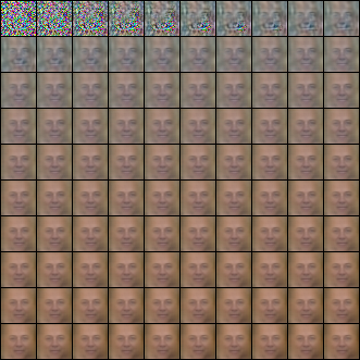
The intuition of using denoisers is this: A good denoiser is specific the distribution of data you're dealing with. It takes any input and moves it to a nearby point that lies in a higher density region. Here is a simple fun example where I train a denoiser neural network on Celeb-A faces. Then I start from random noise (top left), apply the denoiser iteratively, over and over again. This process quickly takes us to high-density region of face-looking things, and eventually converges to a fix-point which is roughly going to be the mode of the distribution:
The converse is also true: if we revert the denoising process by stepping in the other direction instead (which would be implemented by applying the function $x - (F(x) - x)$, where $F$ is the denoiser) we can make faces look less like other faces. We walk away from high-probability regions of the space. This is how denoisers work for maximising the entropy of the variational distribution: they try to push every synthetic sample $G(z; \phi)$ less like one another.
So the denoiser-based variational inference procedure works by training a denoiser, which is used to stretch the variational distribution as wide as possible, while the likelihood and prior terms ensure that the variational posterior is still consistent with the forward model and with observations.
Does this work?
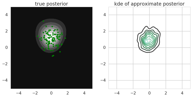
Yes it does, at least on the Bayesian logistic regression toy problem. Here is my Jupyter notebook for this one. The main result is this one (again, you can probably use better models and run this for longer for a nicer result, but it's kind of OK):
Here's another interesting figure to look at: gradients from different components of the loss function: entropy of Q, log prior and log likelihood. Here I'm plotting a quiver plot of negative gradients so you can see which way gradient descent will try to push each sample:
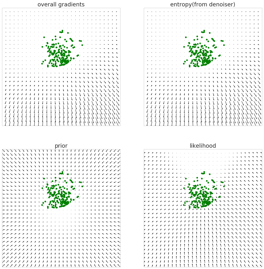
Note that the arrow lengths are normalised for each subplot separately, so they're not comparable.
Or, a better way to plot this, putting arrows only around samples (now the arrow lengths are comparable across subplots):
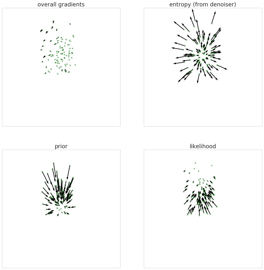
As you can see the entropy component (which comes from the denoiser) tries to stretch the distribution out as wide as possible. The prior tries to contract it and move it closer to the mean, which I chose to be $0$. The likelihood tries to make everything go North as these parameter values are more compatible with the data.
At equilibrium these gradients eventually cancel each other as the variational posterior approaches the real posterior (assuming it can be represented by the variational distribution).
Implementation details
The hard bit to implement is perhaps the custom backpropagation of the denoiser output as gradients. Here I made use of theano's helpful Lop function. Here's what I did:
First, I calculate the derivative of the entropy with respect to samples, as in the formula above. In this, samples_from_generator is basically $x$ and denoised_samples_from_generator are $F(x)$:
dHdG = (samples_from_generator - denoised_samples_from_generator)/noise_variance_var
Then here I calculate the derivative of the entropy with respect to $\phi$ by invoking the chain rule. I had to flatten the tensors because 'Lop' only works when $f$ is a vector, and here samples_from_generator is a matrix. Also, I had to divide by batchsize_var as this will calculate the sum, rather than the mean over the first axis:
dHdPhi = T.Lop(
    f = samples_from_generator.flatten()/batchsize_var,
    wrt = params_G,
    eval_points=dHdG.flatten())
The final detail that may need explaining is that when usign lasagne.updates.adam I passed it a list of pre-computed gradients $dLdPhi$ rather than the loss function itself. In fact, the loss function value is never even computed, only its gradient:
updates_G = adam(
    dLdPhi,
    params_G,
    learning_rate=learningrate_var,
)
Reconstruction error ≠ energy
Why did I write the equations above in such a complicated way? Why do I talk about the gradient of the entropy rather than the entropy itself? The reason is, while the gradients work out fine, it's quite hard to express the energy (log density) itself. People often use the mean squared reconstruction error $|F(x) - x|^2$ as a proxy to energy. However, as pointed out by Alain and Bengio, (2014), this contradicts the connection to the gradients. Let's see what the gradients of the reconstruction error would be:
$$
\frac{\partial}{\partial x} c|F(x) - x|^2 = 2c(F(x) - x)(F'(x) - I)
$$
However, we also know that in the limit of low noise
$$
\frac{\partial}{\partial x} E(x) \approx \frac{1}{\sigma_n^2}(F(x) - x)
$$
Unless $F'(x) - I$ is constant, the two gradients don't match up. If $F$ is approximately the gradient of the energy then $F'(x)$ is its Hessian. The Hessian is constant only if the energy is quadratic, which happens if the distribution - in our case $q$ - is Gaussian. So for Gaussian distributions it's OK to interpret the reconstruction error as the energy, but for others it's not.
This complicates some things when using denoisers in the context of either VI or generative modelling. Instead of simply backpropagating through a nice function, we need to do weird things with the gradients. There are multiple ways of doing it, in the notebook I use one way.
Related papers
This method has been used a few times. For example in this talk (my bit starts around 20:00 but the others are great talks, too.) I proposed a new class of GAN-like algorithms for generative modelling that I called DGGM or denoiser-guided generative models. This idea never made it into a paper (or even a blog post), and never made it work particularly well for generative modelling (didn't try very hard). We then used a variant of the idea in (Sønderby et al, 2016) in the context of image superresolution for amortised MAP inference. As far as we're aware this was the first use of this technique where we backpropagate the output of a separately trained denoiser to train probabilistic models for variational inference. Please do jump in and Schmidhuber me if there are other papers that do exactly this, as I'm sure there will be.
There is also a related ICLR submission by Warde-Farley and Bengio (2016) on denoising feature matching that makes use of denoisers for generative modelling - together with the usual GAN scenario. However, they perform denoising in a nonlinear feature space, which breaks the exact math somewhat (see their Section 3.1 to understand this better).
Energy-based GANs (Zhao et al) also make reference to the same observation: that denoising autoencoders can learn energy functions. However, as I understood from Yann LeCun's talk at the NIPS workshop, when they talk about energy functions they don't mean log densities, they mean any function that has low values around datapoints and high values elsewhere. As such, they rather liberally change the objective functions in ways that - although they guarantee a Nash equilibrium - loose connections to probabilistic or information theoretic quantities. Therefore, these themselves are not applicable to express exact variational lower bounds for example.
Denoisers feature often in the excellent work of Harri Valpola and colleagues. See for example the ladder networks (Rasmus et al, 2015) or their latest work on perceptual grouping. (Greff et al, 2016).
Finally, let me point out that as Alain and Bengio, (2014) show, one can also use regularised autoencoding rather than denoising as a surrogate task to achieve the same properties. Here, I've explained everything in terms of denoising as it is conceptually nice, but it is quite likely that the regularised objective works better in practice not least because there is less random sampling going on.
Summary
In previous posts in this series I have shown how to use logistic regression as a density ratio estimator in the context of variational inference. One can do a lot with those kinds of algorithms. And logistic regression is just one - but not the only one - example of direct density ratio estimation, there are several other examples, for example in the work of Shugiyama and collagues.
Here, I have shown an alternative to density ratio estimation. Instead of estimating ratios, we estimate gradients of log densities. For this, we can use denoising as a surrogate task.
OK, but why???
So why did I do this? The usual answer from a machine learning research is: because I can. This is going to be yet another tool we can use to deal with implicit probabilistic models for inference and learning, whether it's superior in any way to discriminator-based techniques remains to be seen.
Pros
- denoisers estimate gradients directly, and therefore we might get better estimates than first estimating likelihood ratios and then taking the derivative of those. Adversarial examples show that neural-network-based discriminators are not very robust with respect to taking gradients, so this may turn out to be a nice
property - allows you to pick and choose which distributions you want to be implicit. In this case I only chose the variational posterior $q$ to be implicit, and everything else is handled explicitly. Generally speaking, if the prior is explicit, it's probably better to use it explicitly rather than implicitly via sampling.
Cons
- the theory holds in the limit of infinitesimally small noise, but in practice denoisers are trained on small noise. This may result in blurring some fine details of the distributions, and we have seen in (Sønderby et al, 2016) that samples from such a model do tend to be blurrier. Moreover, the denoising objective relies on sampling, which is inefficient in high dimmensions. To solve both problems, the regularised autoencoder might be a better option.
- the denoiser function is only accurate around the support of the distribution. Far away from samples, the denoising function is never trained and can develop spurious modes. One can address this by taking an ensemble of denoisers, and only accepting a high gradient signal if all ensemble members agree on the direction. But generally speaking, denoising isn't accurate far away from samples, and this is where discrimination might be somewhat better.