Variational Inference using Implicit Models Part III: Joint-Contrastive Inference, ALI and BiGAN
This post is part of a series of tutorials on how one can use implicit models for variational inference. Here's a table of contents:
- Part I: Inference of single, global variable (Bayesian logistic regression)
- Part II: Amortised Inference via the Prior-Contrastive Method (Explaining Away Demo)
- ➡️️Part III (you are here): Amortised Inference via a Joint-Contrastive Method (ALI, BiGAN)
- Part IV : Using Denoisers instead of Discriminators
This post is a short follow-up to Part II, showing a different way in which adversarial-like algorithms can be used to approximate variational inference with implicit models. As a reminder, we're interested in inference in a latent variable model, where for each i.i.d. observation $y_n$ we have an associated latent variable $x_n$
Recap on variational inference
Skip this if you know this. Here's the notation I use:
- $p(x)$ is the prior
- $p(y\vert x)$ is the likelihood
- $p(x\vert y)$ is the posterior, which is intractable
- $q(x\vert y)$ is the recognition model which is meant to approximate the posterior
- $p_{0}(y)$ is the real distribution from which data is drawn from. In statistics this would be called the population distribution. This is constant and unknown.
- $p_{\mathcal{D}}$ is the empirical distribution of observed data $\mathcal{D}$, which is essentially a collection of point masses $p_{\mathcal{D}}(y) = \frac{1}{N}\sum_{n=1}^{N}\delta(y-y_n)$
In variational inference we are interested in minimising the following divergence:
$$
\mathbb{E}_{y \sim p_0} \operatorname{KL}[ q(x \vert y) | p(x \vert y)]
$$
We can rearrange this in the following way:
\begin{align}
\mathbb{E}_{y \sim p_0} \operatorname{KL}[ q(x \vert y) | p(x \vert y)] &= \mathbb{E}_{y\sim p_0} \mathbb{E}_{x\vert y \sim q(x\vert y)} \log \frac{q(x\vert y)}{p(x\vert y)}\\
&= \mathbb{E}_{y\sim p_0} \mathbb{E}_{x\vert y \sim q(x_ y)} \log \frac{q(x\vert y)p(y)}{p(y\vert x)p(x)} + \mathbb{E}_{y\sim p_0}\log p_0(y) - \mathbb{E}_{y\sim p_0}\log p_0(y)\\
&= \mathbb{E}_{y\sim p_0} \mathbb{E}_{x\vert y \sim q(x_ y)} \log \frac{q(x\vert y)p_0(y)}{p(y\vert x)p(x)} + \mathbb{E}_{y\sim p_0} \frac{\log p(y)}{\log p_0(y)}\\
&= \operatorname{KL}[ q(x \vert y) p_0(y)| p(x, y)] - \operatorname{KL}[p_0(y)|p(y)]
\end{align}
In the second line I used Bayes' rule, and added and substracted the same quantity. We can write this equation as a bound:
$$
\mathcal{L}(q) = \operatorname{KL}[ q(x \vert y) p_0(y)| p(x, y)] = \operatorname{KL}[p_0(y)|p(y)] + \mathbb{E}_{y \sim p_0} \operatorname{KL}[ q(x \vert y) | p(x \vert y)] \geq \operatorname{KL}[ q(x \vert y) | p(x \vert y)]
$$
The right hand-side of this boind is the KL divergence between the real data distribution $p_0(y)$ and the marginal likelihood $p(y)$. This is exactly what we would like to minimize in maximum likelihood training and indeed this is closely related to the likelihood. The left-hand side is the (negative) variational lower bound. The bound is exact if the $\mathbb{E}_{y \sim p_0} \operatorname{KL}[ q(x \vert y) | p(x \vert y)]$ term is $0$, which only happens if $q(x \vert y)$ matches the posterior perfectly.
Joint-contrastive method
As the derivation above suggests, the variational bound can be expressed as the expectation of the following logarithmic density ratio:
$$
\mathcal{L}(q) = \mathbb{E}_{y\sim p_0} \mathbb{E}_{x\vert y \sim q(x\vert y)} \log \frac{q(x\vert y)p(y)}{p(y\vert x)p_0(x)}
$$
Note that in practice we approximate sampling from $p_0$ by sampling datapoints from $p_\mathcal{D}$ instead. As in Part II, we are going to approximate this density ratio with a discriminator $D(x, y)$ trained via logistic regression. As before, the discriminator will take an $(x, y)$ pair. Whereas in Part II this was our choice (remember, we amortized the discriminator) now it is absolutely essential. Once we introduce the discriminator we obtain the following two-step iterative algorithm:
First, we minimise the discriminator loss, keeping the generator $G$ fixed:
$$
\mathcal{L}(D; G) = \frac{1}{N} \sum_{n=1}^{N} \mathbb{E}_{x\sim q(x \vert y_n)} \log D(x,y_n) + \mathbb{E}_{x\sim p(x)}\mathbb{E}_{y\vert x \sim p(y\vert x)} \log (1 - D(x, y))
$$
Then we improve the generator using the following loss (exactly as before):
\begin{align}
\mathcal{L}(G; D) &= \frac{1}{N} \sum_{n=1}^{N} \mathbb{E}_{x\sim q(x\vert y_n)} \left[ \log \frac{D(x, y_n)}{1 - D(x, y_n)}\right]\\
&= \frac{1}{N} \sum_{n=1}^{N} \mathbb{E}_{z\sim\mathcal{N}(0,I)} \left[ \log \frac{D(G(z,y_n), y_n)}{1 - D(G(z,y_n), y_n)}\right]
\end{align}
So in the first step, given the generator $G$ we train a discriminator $D$ to classify $(x,y)$ pairs. The pairs are sampled as follows:
- for real examples we take a real datapoint $y_n$ and infer the corresponding latent using our recognition model $q(x\vert y_n)$.
- for synthetic samples we draw $x$ from the prior $p(x)$, and simulate $y$ from the forward model $p(y\vert x)$. This is the same as saying that the pair $(x,y)$ are drawn from the joint $p(x,y)$.
Compared with the amortized scheme of Part II, there are two differences:
- the way $y$ is sampled for synthetic examples is different. Previously, $y$ was always a real datapoint. Here, for synthetic samples it is sampled conditionally on $x$.
- the likelihood $p(y\vert x)$ doesn't appear in the generator's training objective anymore. This means that the likelihood can also be implicit now, just as the prior $p(x)$ and the recognition model $q(x\vert y)$.
In the prior-contrastive scheme $y$ was only provided to the discriminator by way of context. As it is always sampled from the same marginal distribution it alone cannot help the discriminator figure out if it is looking at a real or a synthetic sample. Indeed, had we decided not to amortise the discriminator in that case, we could have trained separate discriminators for each $y_n$.
In contrast, I call this method joint-contrastive inference as the discriminator learns to contrast joint distributions $p(x,y)$ and $q(x\vert y)p_0(y)$. Here, $y$ is sampled differently for the real and synthetic pairs, so the discriminator can and should learn to discriminate on the basis of $y$.
If everything converges, the discriminator converges to a constant $0.5$. It's easy to see why: Suppose our model describes the world perfectly, and the approximate posterior mimicks the real posterior perfectly. Then, there should be no difference between first sampling an $x$ and then a $y$ from the model, or first sampling a $y$ from the world and subsequently inferring $x$. This is the kind of Nash equilibrium we are hoping to reach.
Connections to ALI, BiGANs
This scheme is almost exactly the same as ALI (Adversarially Learned Inference, Dumoulin et al, 2016) or BiGANs (Donahue et al, 2016). These papers independently discovered the same algorithm and it happens to work very well. As far as I'm aware neither papers provide a derivation of these algorithms from first principles like above, and neither papers used the KL-divergence loss function to make the connection to variational inference valid. So now you know: ALI and BiGAN (can be modified to) approximate maximum likelihood learning.
I should mention that the notation and terminology used in those papers is very different from how I presented things here. They call the generator $G$ which defines auxillary distribution $q$ the encoder for example. But identifying the components should be pretty straightforward.
The main difference from what is presented here is the specific form of the generator loss used to update $q$. In these papers the authors use the form that approximates the Jensen-Shannon divergence between $p(y, x)$ and $q(x\vert y)p_0(y)$, but to obtain the variational bound we have to use the loss function that corresponds to the $\operatorname{KL}$ divergence (Sønderby et al, 2016).
Hierarchical models
Just as VAEs, one can stack multiple instances of the variational BiGAN on top of one another. As I mentioned earlier, maximising variational lower bound with respect to the prior $p(x)$ is the same as fitting $p(x)$ to data sampled from the aggregate posterior $\frac{1}{N} \sum_{n=1}^{N} q(x\vert y_n)$ via maximum likelhiood. This can be seen by observing:
\begin{align}
\mathbb{E}_{y \sim p_0} \operatorname{KL}[ q(x \vert y) | p(x \vert y)] &= \mathbb{E}_{y \sim p_0} \mathbb{E}_{x\vert y \sim p(x\vert y)} \log \frac{ q(x \vert y) }{ p(x \vert y) } \\
&= \mathbb{E}_{y \sim p_0} \mathbb{E}_{x\vert y \sim p(x\vert y)} \log \frac{ q(x \vert y) p(y)}{ p(x) p(y\vert x)} \\
&= - \mathbb{E}_{y \sim p_0} \mathbb{E}_{x\vert y \sim p(x\vert y)} \log p(x) + c
\end{align}
This means that, if $p(x)$ is a hierarchical model in itself, we can lower bound the lower bound with respect to parameters of $p(x)$ using variational inference. Here's a diagram I drew to illustrate this:
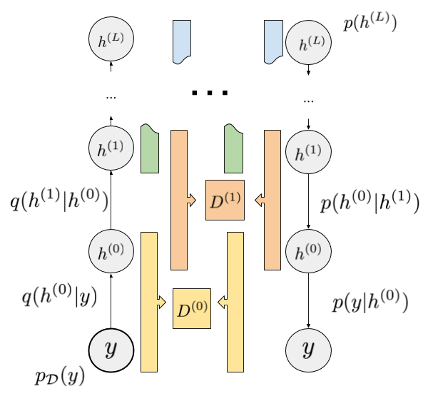
The model has layers of hidden variables $h^{(0)}$ all the way up to $h^{(L)}$. On the right, we have a prior on $h^{(L)}$ and set of forward models $p(h^{(\ell-1)}\vert h^{(\ell)})$, finally a forward model of observations conditioned on the lowest layer $p(y\vert h^{(0)})$.
All of these can be implicit models.
On the left we have the recognition pathway. Here, $y$ is sampled from the empirical data distribution $p_{\mathcal{D}}$, and subsequent layers are sampled from the recognition models $q(h^{(\ell)} \vert h^{(\ell - 1)})$.
All recognition models can be implicit, too.
For each pair of neighbouring layers we have discriminators $D^{(\ell)}$ which are trained to classify $(h^{(\ell-1)},h^{(\ell)})$ pairs from the left-hand inference stream vs the right-hand generative stream. Once the discriminators are converged, the recognition models $q$ and all the forward models $p$ can be updated jointly by maximising the variational lower bound that corresponds to that layer.
A drawback of this hierarchical model is that as we go up in the layer hierarchy our lower bounds get weaker and weaker. Also, such model with implicit models everywhere, might prove to be way too complicated to learn meaningful feature hierarchies. The lower layers themselves could do much of the job if they are allowed to be complex enough.
Finally, as pointed out in (Ladder Variational Autoencoders, Sønderby et al, 2016b], stacked recognition models that only depend on the layer below may not be the best way to approximate inference. They instead introduce inference models that take into account upstream and downstream dependencies simultaneously, which kind of makes sense. I am unsure whether this ALI/BiGAN method could apply in that situation, but I'll leave that for you as homework.
Summary
In this part of my mini-series on variational inference with implicit models I covered a method I call joint-contrastive learning. It is closely related to existing methods ALI and BiGAN, but it is motivated from first principles and it can be shown that it approximates variational inference and learning.
Unlike in previous methods, now all the distributions involved, including the prior, likelhiood and recongition models, can be implicit. We only ever need to (a) sample from these distributions, and (b) evaluate the gradient of the expectations with respect to model parameters.
On one hand, This makes this approach super versatile as we can plug in a wide range of stochastic neural networks or probabilistic programs and in theory the whole thing just works. We can also stack these things on top of one another and the theory still works out. On the other hand, it makes me wonder whether this flexibility comes at a price. Conventional thinking is that if your assumptions about your generative models are too loose and permissive, the inference method will be able to exploit that flexibility and overfitting could occur. Technically, the method allows you to plug in arbitrarily large neural networks everywhere. But perhaps a better way forward is to keep your forward models highly structured and informed. For visual perception, I would look at (Kulkarni et al, 2015) for inspiration.