Variational Inference using Implicit Models Part II: Amortised Inference
This post is part of a series on Variational Inference with Implicit Models. Here is a table of contents:
- Part I: Introduction, Inference of single, global variable (Bayesian logistic regression)
- ➡️️Part II (you are here): Amortised Inference via the Prior-Contrastive Method (Explaining Away Demo)
- Part III: Amortised Inference via a Joint-Contrastive Method (ALI, BiGAN)
- Part IV: Using Denoisers instead of Discriminators
GHOST_URL/variational-inference-using-implicit-models-part-iv-denoisers-instead-of-discriminators/
In a previous post I showed a simple way to use a GAN-style algorithm to perform approximate inference with implicit variational distributions. There, I used a Bayesian linear regression model where we aim to infer a single global hidden variable given a set of conditionally i.i.d. observations. In this post I will consider a slightly more complicated model with one latent variable per observation, and just like in variational autoencoders (VAEs), we are going to derive an amortised variational inference scheme.
The graphical model now looks like this:
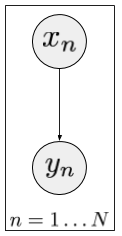
For each observation $y_n$ there is an associated latent variable $x_n$, which are drawn i.i.d. from some prior $p(x)$.
As for the notation: the $x$ for latents, $y$ for observed data notation is used in some old-school statistical ML literature such as my favourite paper - in the GAN/VAE literature, my $x$ would be a $z$ and my $y$ would be an $x$. Sorry for the confusion, I wrote it this way, but I should probably adapt to the times at some point and update my notation
Variational inference in such model would involve introducing variational distributions $q_n(x)$ for each observation $y_n$, but doing so would require a lot of parameters, growing linearly with observations. Furthermore, we could not quickly infer $x$ given a previously unseen observation. We will therefore perform amortised inference where we introduce a recognition model $q(x_n\vert y_n; \psi)$, parametrised by the observation $y$, and only adjust a single set of parameters $\psi$ that is shared across all observations. In the following I will omit the parameter $\psi$ and just refer to the variational distribution as $q(x_n\vert y_n)$.
A summary of this post
- I look at using an implicit $q(x_n\vert y_n)$ for VI: one we can sample from but whose density we cannot evaluate
- there are (at least) two ways of doing this using GAN-style algorithms which involves a discriminator
- here, I will focus on what I call prior contrastive inference, in which we estimate the average density ratio between the prior and the variational distribution
- we need one discriminator per observation, so we are going to amortise the discriminator, too.
- I introduce a simple toy model following the well-known sprinkler-rain anecdote which exhibits explaining away.
- I implement the prior-contrastive inference method on this toy problem (with an iPython notebook)
- as it turns out what I did is pretty much the same as this brand new arXiv paper by Mescheder et al. 2017, so go read that paper, too.
- there is a second way to derive a GAN-type algorithm from first principles in this context. This leads to an algorithm similar to ALI (Dumoulin et al, 2016) and BiGAN (Donahue et al, 2016). I will leave this as homework for you to figure out, and will cover in more detail in a future post.
Take a step back: Why?
A question I never really went into in the previous post is: why do we even want to perform variational inference with implicit models? There can be many reasons but perhaps most importantly, we can model more complicated distributions with implicit models. In normal VI we are often limited to exponential family distributions such as Gaussians. When dealing with joint distributions we often approximate these with products of independent factors. Even in VAEs, although the recognition model can be a very complex function of its input, at the end of the day we usually outputs just a single Gaussian. We are interested in improving approximate inference in models whose posteriors will be very complicated, maybe multimodal, or concentrated on a manifold, or handle weird shapes that arise when dealing with non-identifiability. The parametric assumptions we make in VI are often too strong, and implicit models would be one way to relax these.
Prior-contrastive discrimination
Let's follow the same footsteps as in the first post and rearrange the KL divergence in terms of the log density ratio between the prior and the approximate posteriors:
$$
\frac{1}{N} \sum_{n=1}^{N} \operatorname{KL}\left[q(x\vert y_n) \middle| p(x\vert y_n) \right] = \frac{1}{N} \sum_{n=1}^{N} \operatorname{KL}\left[q(x\vert y_n) \middle| p(x) \right] - \frac{1}{N} \sum_{n=1}^{N} \mathbb{E}_{x \sim q(x\vert y_n)} \log p(y_n \vert x) + p(y_{1\ldots N})
$$
As a reminder, $q(x\vert y)$ is an implicit recognition model, so we need a method for estimating the logarithmic density ratio $q(x\vert y_n)/p(x)$ for any observation $y$. Again, we can use logistic regression to do this, introducing a discriminator. I call this approach prior-contrastive as the discriminator will learn the contrast between $q$ and the prior.
As for the discriminator, we could either
- train one logistic regression discriminator $D_n(x)$ for each observation $y_n$, or
- amortise the discriminator, that is learn a logistic regression classifier $D(x, y)$ that takes a $y$ as input in addition to $x$.
We will follow the second option to obtain the following iterative algorithm:
Discriminator loss:
$$
\mathcal{L}(D; G) = \frac{1}{N} \sum_{n=1}^{N} \mathbb{E}_{x\sim q(x \vert y_n)} \log D(x,y_n) + \mathbb{E}_{x\sim p(x)} \log (1 - D(x, y_n))
$$
Generator loss:
\begin{align}
\mathcal{L}(G; D) &= \frac{1}{N} \sum_{n=1}^{N} \mathbb{E}_{x\sim q(x\vert y_n)} \left[ \log \frac{D(x, y_n)}{1 - D(x, y_n)}- \log p(y_n \vert x)\right]\\
&= \frac{1}{N} \sum_{n=1}^{N} \mathbb{E}_{z\sim\mathcal{N}(0,I)} \left[ \log \frac{D(G(z,y_n), y_n)}{1 - D(G(z,y_n), y_n)}- \log p(y_n \vert x)\right]
\end{align}
So in the first step, given the generator $G$ we train a discriminator $D$ to classify $(x,y)$ pairs, where $y$ is always a real datapoint and $x$ is sampled either conditionally using the recognition model, or independently, from the prior. Then, keeping the discriminator fixed, we take a single gradient step to improve the generator.
I note here that the generator's loss function is an approximation to the variational lower bound (with a minus sign), so we can minimise the same loss with respect to parameters of $p(y\vert x)$ to obtain a VAE-like learning algorithm. If we do this, assuming that the generator and discriminator can be perfect all the time, this provides us a way to perform approximate maximum likelihood. In what follows, I will only care about approximate inference in a fixed model.
Simple Demo: Explaining Away
To demonstrate that this method works, I coded up a simple toy model, which has 2-dimensional real-valued latent variables ($x_n$) and univariate positive real observations ($y_n$).
It's the simplest model I could come up with which exhibits explaining away: The prior on the two latent features is independent, but conditioned on the observation, the latent features become dependent. Explaining Away is a super-important pattern for inference, there are lots of sources to read up on it if you're not familiar with it.
My simple explaining away model looks like this:
\begin{align}
x &\sim \mathcal{N}(0, \sigma^2 I)\\
y\vert x &\sim \operatorname{EXP}(3 + max(0,x_1)^3 + max(0,x_2)^3),
\end{align}
where $\operatorname{EXP}(\beta)$ denotes an exponential random variable with mean $\beta$, and $max(0,x_1)$ is better known as ReLU. Basically what's happening here: if either $x_1$ or $x_2$ has a large value, we observe a higher $y$ value. To connect this to the usual sprinkler example: if $x_1$ is the sprinkler, $x_2$ is the rain, and $y$ the wetness of the grass.
Here is what the (unnormalised) posteriors $Zp(x\vert y)$ look like for different values of $y$:
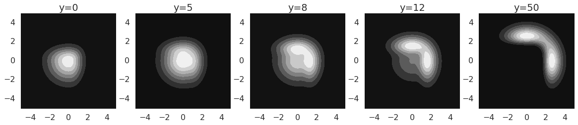
One can see that these posteriors are multimodal and oddly shaped, so trying to match them with a Gaussian - which is what the simplest variational method would do - would likely fail to capture everything that is going on. So this is a simple but great example (I think) of a situation where we might need flexible approximate posteriors.
Let's see how well this works
I have coded up the prior-contrastive method above to perform approximate inference in the explaining away toy model. As before, I am sharing an iPython notebook, which is perhaps even messier than before, but hopefully still useful for most of you.
Here are the approximate posteriors I got, using this simple method (the bottom row shows the real posteriors, for reference):
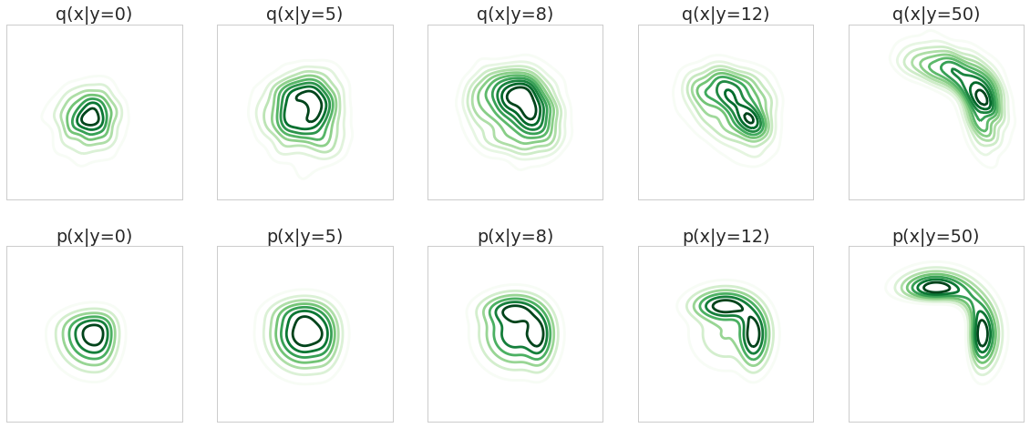
these results are far from perfect, it doesn't quite capture the symmetry of the problem, and it only partially models the multimodality of the $y=50$ case, but it does a decent job. Let me also say that I spent very little time actually trying to make this work, and I would expect it to work much better when given appropriate care - probably in the form of better models for both $q$ and $D$.
As I noted in the previous post, we also know what the discriminator should converge to, and we expect $\Phi^{-1}(D(x,y))$ to converge to the log-likelihood $p(y\vert x)$ up to a constant. Here is what these unnormalised discriminators look like (top) compared to what we expect them to be (bottom):
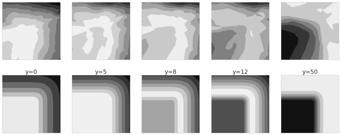
Again, these are far from perfect, but I'd say they look qualitatively OK.
Related Papers
Between writing this, and publishing it, there's a paper on arXiv that does more or less the same thing:
- Mescheder, Nowozin and Geiger (2017) Adversarial Variational Bayes: Unifying Variational Autoencoders and Generative Adversarial Networks.
Please go read that paper for a proper experiments and more details on derivations.
This technique is similar to ALI (Dumoulin et al, 2016) and BiGAN (Donahue et al, 2016), two independently discovered versions of the same algorithm. They, too, train a discriminator on $(x,y)$ pairs, but while in the method I showed you here $y$ is always a real datapoint, in ALI and BiGAN, in one class it is sampled conditionally given $x$ using the likelihood $p(y\vert x)$. They also don't have the extra likelihood term that we have when train $q$.
This is also related to AffGAN (Sønderby et al, 2016) which is derived for image superresolution. The main difference there is that the likelihood is degenerate, and the $q$ network is designed so that the likelihood of its output is constant. This simplifies a number of things: Firstly, the discriminator no longer has to take $(x,y)$ pairs, it only works on $x$. Secondly, the likelihood term in the generator's loss is constant so it can be omitted.
Summary
Here I've shown a method for amortised variational inference using implicit variational distributions. I have simply expressed the variational lower bound in terms of the logarithmic probability ratio between the variational distributions $q(x\vert y)$ and the prior $p(x)$, and I used logistic regression to approximate this density ratio from samples. This gives rise to a GAN-style algorithm where the discriminator $D(x,y)$ discriminates between $(x,y)$ pairs. For both classes, $y$ is drawn from the dataset, for the synthetic class, $x$ is generated conditionally using the recongintion model, while for the "real" class, $x$ is sampled from the prior. I called this the prior-contrastive approach.
Hierarchical models
One can see that in order to maximise the variational bound with respect to parameters of the prior $p(x)$, one has to minimise $\operatorname{KL}[\hat{q}(x)\vert p(x)]$, where $\hat{q}(x) = \frac{1}{N} q(x\vert y_n)$ is the aggregate posterior. This is the same as maximum likelihood learning, where we want to fit $p(x)$ onto data sampled from $\hat{q}(x)$. We can therefore make $p(x)$ a latent variable model itself, and repeat the variational inference method to create a hierarchical variational model.
Criticism
There are a few problems with this approach:
- As before, the posterior is likely to be quite dissimilar from the prior, which might mean that the estimate of the discriminator loss will require too many samples to provide meaningful gradients. Logistic regression works best for density ratio estimation when the distributions are similar.
- This method still requires the likelihood $p(y\vert x)$ to be analytical, while $p(x)$ and the variational posterior $q(x\vert y)$ can be implicit. This method doesn't work if $p(y\vert x)$ itself is implicit. By contrast, methods like ALI or BiGAN relax even this requirement.
Homework #1
As I'm now home with my newborn daughter (shoutout to twitter for their amazing employee benefits which includes the industry's best parental leave program) I don't have much time to work out details myself, so in the spirit of learning, I'll give you homework.
First one: vanilla VAE can be reproduced as a special case of this. Try to modify the code so that $q(x\vert y)$ is more like the VAE Gaussian recognition model. You only need to change the network by moving the noise at the very end, mimicking the reparametrisation trick. Run the thing and see what you get. My bet is a lopsided approximate posterior: it will learn one of the posterior modes and ignore the other mode completely.
Homework #2
What's the next step from this? As I already mentioned, there is another way to express the variational bound in terms of a KL divergence, and if one uses logistic regression to estimate relevant log density ratios, one gets an alternative GAN-type algorithm. I already gave you a clue in the intro saying that the resulting algorithm will look a lot like ALI or BiGAN. Off you go.
Finally, thanks to Ben Poole for some comments on this draft, and for pointing out the new paper by Mescheder and colleagues.