Autoregressive Models, OOD Prompts and the Interpolation Regime

A few years ago I was very much into maximum likelihood-based generative modeling and autoregressive models (see this, this or this). More recently, my focus shifted to characterising inductive biases of gradient-based optimization focussing mostly on supervised learning. I only very recently started combining the two ideas, revisiting autoregressive models throuh the lens of inductive biases, motivated by a desire to understand a bit more about LLMs. As I did so, I found myself surprised by a number of observations, which really should not have been surprising to me at all. This post documents some of these.

AR models > distributions over sequences

I have always associated AR models as just a smart way to parametrize probability distributions over multidimensional vectors or sequences. Given a sequence, one can write

$$
p(x_1, x_2, \ldots, x_N;\theta) = \prod_{n=1}^{N} p(x_n\vert x_{1:n-1}, \theta)
$$

This way of defining a parametric joint distribution is computationally useful because it is significantly easier to ensure proper normalization of a conditional probability over a single variable than it is to ensure proper normalization over a combinatorially more complex space of entire sequences.

In my head, I considered there to be a 1-to-1 mapping between autoregressive models (a family of conditional probabilities $\{p(x_n\vert x_{1:n-1}), n=1\ldots N\}$) and joint distributions over sequences $p(x_1,\ldots,x_N)$. However, I now understand that is, generally, a many-to-one mapping.

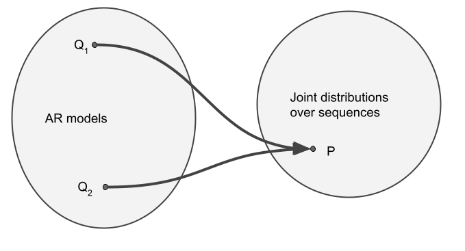
Why is this the case? Consider a distribution over two binary variables $X_1$ and $X_2$. Let's say that, $\mathbb{P}(X_1=0, X_2=0) = \mathbb{P}(X_1=0, X_2=1) = 0$, meaning that $\mathbb{P}(X_1=0)=0$, i.e. $X_1$ always takes the value of $1$. Now, consider two autoregressive models, $Q_1$ and $Q_2$. If these models are to be consistent with $P$, they must agree on some facts:

• $\mathbb{Q}_1[X_2=x\vert X_1=1] = \mathbb{Q}_2[X_2=x\vert X_1=1] = \mathbb{P}[X_2=x\vert X_1=1] = \mathbb{P}[X_2=x]$ and
• $\mathbb{Q}_1[X_1=1] = \mathbb{Q}_2[X_1=1] = 1$.

However, they can completely disagree on the conditional distribution of $X_2$ given that the value of $X_1$ is $0$, for example $\mathbb{Q}_1[X_2=0\vert X_1=0] =1$ but $\mathbb{Q}_2[X_2=0\vert X_1=0] =0$. The thing is, $X_1$ is never actually $0$ under either of the models, or $P$, yet both models still specify this conditional probability. So, $Q_1$ and $Q_2$ are not the same, yet they define exactly the same joint distribution over $X_1$ and $X_2$.

Zero probability prompts

The meaning of the above example is that two AR models that define exactly the same distribution over sequences can arbitrarily disagree on how they complete $0$-probability prompts. Let's look at a more language modely example of this, and why this matters for concepts like systemic generalisation.

Let's consider fitting AR models on a dataset generated by a probabilistic context free grammar $\mathbb{P}[S=\"a^nb^n\"]=q^n(1-q)$. To clarify my notation, this is a distribution over sentences $S$ that take are formed by a number of `a` characters followed by the same number of `b` charactes. Such a langauge would sample $ab$, $aabb$, $aaabbb$, etc, with decreasing probability, and only these.

Now consider two autoregressive models, $Q_1$ and $Q_2$, which both perfectly fit our training distribution. By this I mean that $\operatorname{KL}[Q_1\|P] = \operatorname{KL}[Q_2\|P] = 0$. Now, you can ask these models different kinds of questions.

• You can ask for a random sentence $S$, and you get random samples returned, which are indistinguishable from sampling from $P$. $Q_1$ and $Q_2$ are equivalent in this scenario.
• You can use a weird sampling method, like temperature scaling or top-p sampling to produce samples from a different distribution than $P$. It's a very interesting question what this does, but if you do this in $Q_1$ and $Q_2$, you'd still get the same distribution of samples out, so the two models would be equivalent, assuming they both fit $P$ perfectly.
• You can ask each model to complete a typical prompt, like $aaab$. Both models will complete this prompt exactly in the same way, responding $bb$ and the end of sequence token. The two models are equivalent in terms of completions of in-distribution prompts.
• You can ask each model to complete a prompt that would never naturally be seen, like $aabab$, the two models are not equivalent. P doesn't prescribe how this broken prompt should be completed as it doesn't follow the grammar. But both $Q_1$ and $Q_2$ will give you a completion, and they may give completely different ones.

When asked to complete an out-of-distribution prompt, how will the models behave? There is no right or wrong way to do this, at least not that one can derive from $P$ alone. So, let's say:

• $Q_1$ samples completions like $\mathbf{aabab}b$, $\mathbf{aabab}bab$, $\mathbf{aabab}bbaba$, while
• $Q_2$ samples $\mathbf{aabab}$, $\mathbf{aabab}bbb$, $\mathbf{aabab}bbbbbb$.

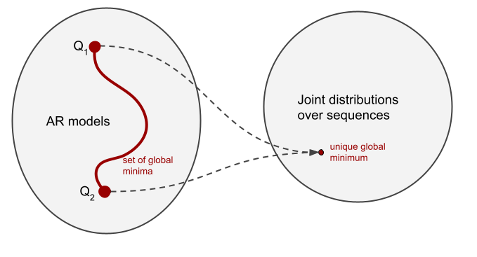
In this example we can describe the behaviour of each of the two models. $Q_1$ applies the rule "the number of $a$s and $b$s must be the same". This is a rule that holds in $P$, so this model has extrapolated this rule to sequences outside of the grammar. $Q_2$ follows the rule "once you have seen a $b$ you should not generate any more $a$s". Both of these rules apply in $P$, and in fact, the context free grammar $a^nb^n$ can be defined as the product of these two rules (thanks to Gail Weiss for pointing this out during her Cambridge visit). So we can say that $Q_1$ and $Q_2$ extrapolate very differently, yet, they are equivalent generative models at least so far as the distribution of sequences is concerned. They both are global minima of the training loss. Which one we're more likely t get as a result of optimization is up to inductive biases. And of course, there's more than just these two models, there are infinitely many different AR models consistent with P that differ in their behaviour.

Consequence for maximum likelihood training

An important consequence of this is that model likelihood alone doesn't tell us the full story about the quality of an AR model. Even though cross entropy is convex in the space of probability distributions, it is not strictly convex in the space of AR models (unless the data distribution places non-zero probability mass on all sequences, which is absolutely not the case with natural or computer language). Cross entropy has multiple - infinitely many - global minima, even in the limit of infinite training data. And these different global minima can exhibit a broad range of behaviours when asked to complete out-of-distribution prompts. Thus, it is down to inductive biases of the training process to "choose" which minima are likelier to be reached than others.

Low probability prompts

But surely, we are not just interested in evaluating language models on zero probability prompts. And how do we even know if the prompts we are using are truly zero probability under the "true distribution of language"? Well, we don't really need to consider truly zero probability promots. The above observation can likely be softened to consider AR models' behaviour on a set of prompts with sufficiently small probability of occurrence. Here is a conjecture, and I leave it to readers to formalize this fully, or prove some simple bounds for this:

Given a set $\mathcal{P}$ of prompts such that $\mathbb{P}(\mathcal{P}) = \epsilon$, it is possible to find two models $Q_1$ and $Q_2$ such that $Q_1$ and $Q_2$ approximate $P$ well, yet $Q_1$ and $Q_2$ give very different completions to prompts in \mathcal{P}.

Consequence: so long as a desired 'capability' of a model can be measured by evaluating completions of an AR model on a set of prompts that occurr with small probability, cross-entropy cannot distinguish between capable and poor models. For any language model with good performance on a limited benchmark, we will be able to find another language model that matches the original on cross entropy loss, but which fails on the benchmark completely.

A good illustration of the small probability prompt set is given by Xie et al (2021)  who interpret in-context learning ability of language models as implicit Bayesian inference. In that paper, the set of prompts that correspond to in-context few-shot learning prompts have vanishing probability under the model, yet the model gives meaningful responses in that case.

Language Models and the Interpolation Regime

Over the years, a large number of mathematical models, concepts and analysis regimes have been put forward in an attempt to generate meaningful explanations of the success of deep learning. One such idea is to study optimization in the interpolation regime: when our models are powerful enough to achieve zero training error, and mimimizing the training loss thus becomes an underdetermined problem. The interesting outstanding question becomes which of the global minima of the training loss our optimization selects.

The scenarios often studied in this regime include regression with a finite number of samples or separable classification where even a simple linear model can reach zero training error. I'm very excited about the prospect of studying AR generative models in the interpolation regime: where cross entropy approaches the entropy of the training data. Can we say something about the types of OOD behaviour gradient-based optimization favours in such cases?