From Autoencoders to Autoregressive Models (Masked Autoencoders ICML Paper)
This is my second favourite paper from ICML last week, and I think the title really does not do it justice. It is a great idea about training rich, tractable autoregressive generative models of data, and doing so by using standard techniques from autoencoder training with dropout.
- Mathieu Germain, Karol Gregor, Iain Murray, Hugo Larochelle (2015): MADE: Masked Autoencoder for Distribution Estimation
Caveat (again): this is not my work, and this blog post does not really add anything new to the paper, only my perspective on it.
Unsupervised learning primer (again)
Unsupervised learning is about modelling the probability distribution $p(\mathbf{x})$ of some data, from which we observe independent samples $\mathbf{x}_i$. Often, the vector $\mathbf{x}$ is high dimensional, such as in images, where different components of $\mathbf{x}$ encode pixel intensities.
Typically, a probability model is specified as $q(\mathbf{x};\theta) = \frac{f(\mathbf{x};\theta)}{Z_\theta}$, where $f(\mathbf{x};\theta)$ is some positive function parametrised by $\theta$. The denominator $Z_\theta$ is called the normalisation constant which makes sure that $q$ is a valid probability model: it has to sum up to one over all possible configurations of $\mathbf{x}$. The central problem in unsupervised learning is that for the most interesting models in high dimensional spaces, calculating $Z_\theta$ is intractable, so crucial quantities such as the model likelihood cannot be calculated and the model cannot be fitted. The community is therefore in search for
- interesting models that have tractable normalisation constants
- fancy methods to deal with intractable models (pseudo-likelihood, adversarial networks, contrastive divergence)
This paper is about the former.
Core ingredient: autoregressive models
This paper sidesteps the high dimensional normalisation problem by restricting the class of probability distributions to autoregressive models, which can be written as follows:
$$q(\mathbf{x};\theta) = \prod_{d=1}^{D} q(x_{d}\vert x_{1:d-1};\theta).$$
Here $x_d$ denotes the $d^{th}$ component of the input vector $\mathbf{x}$. In a model like this, we only need to compute the normalisation of each $q(x_{d}\vert x_{1:d-1};\theta)$ term, and we can be sure that the resulting model is a valid model over the whole vector $\mathbf{x}$. But as normalising these one-dimensional probability distributions is a lot easier, we have a whole range of interesting tractable distributions at our disposal.
Training multiple models simultaneously
Autoregressive models are used a lot in time series modelling and language modelling: hidden Markov models or recurrent neural networks are examples. There, autoregressive models are a very natural way to model data because the data comes ordered (in time).
What's weird about using autoregressive models in this context is that it is sensitive to ordering of dimensions, even though that ordering might not mean anything. If $\mathbf{x}$ encodes an image, you can think about multiple orders in which pixel values can be serialised: sweeping left-to-right, top-to-bottom, inside-out etc. For images, neither of these orderings is particularly natural, yet all of these different ordering specifies a different model above.
But it turns out, you don't have to choose one ordering, you can choose all of them at the same time. The neat trick in the masking autoencoder paper is to train multiple autoregressive models all at the same time, all of them sharing (a subset of) parameters $\theta$, but defined over different ordering of coordinates. This can be achieved by thinking of deep autoregressive models as a special cases of an autoencoder, only with a few edges missing.
Consider a fixed ordering of input dimensions. Now take a fully connected autoencoder, which defines a probability distribution $q(\hat{\mathbf{x}}\vert\mathbf{x};\theta)$. You can write this as
$$q(\hat{\mathbf{x}}\vert\mathbf{x};\theta) = \prod_{d=1}^{D} q(\hat{x}_{d}\vert x_{1:D};\theta)$$
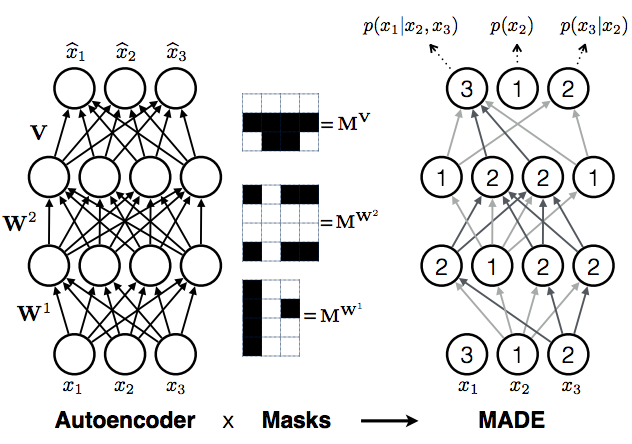
Note the similarity to the autoregressive equation above, the only difference being that each coordinate now depends on every other coordinate ($x_{1:D}$), rather than only coordinates that precede it in the ordering ($x_{1:d-1}$). To turn this equation into autoregressive equation above, we simply have to remove dependencies of each output coordinate $\hat{x}_{d}$ on any input coordinate $\hat{x}_{e}$, where $e>=d$. This can be done by removing edges along all paths from the input coordinate $\hat{x}_{e}$ to output coordinate $\hat{x}_{d}$. You can achieve this cutting of edges by multiplying the weight matrices $\mathbf{W}^{l}$of the autoencoder neural network elementwise by binary masking matrices $\mathbf{M}^{\mathbf{W}^{l}}$. Hence the name masked autoencoder.
The procedure above considered a fixed ordering of coordinates. You can repeat this process for any arbitrary ordering, for which you obtain different masking matrices but otherwise the same procedure. If you train this autoencoder network with randomly sampled masking matrices, you essentially train a family of autoregressive models, each sharing some parameters via the underlying autoencoder network.
Because masking is similar to the popular dropout training, implementing it is relatively straightforward and requires minimal change to existing autoencoder code. However, now you have a generative model - in fact, a large set of generative models - which has a lot of nice properties for you to enjoy.
The slight concern
Of course, this would be all too good to be true: a powerful deep generative model that is easy to evaluate and all. I think the problem with this is the following: If you train just one of these autoregressive models, that's tractable, exact and fine. But you really want to combine all (or many) of these becuause individually they are weak.
What is the interpretation of training with randomly drawn masking matrices? You can think of it as stochastic gradient descent on the following objective:
$$\mathbb{E}_{\mathbf{x}\sim p}\mathbb{E}_{\pi \sim U} \log q(\mathbf{x},\pi,\theta)$$
Here, I used $\pi$ to denote a permutation of the coordinates, and $\mathbb{E}_{\pi \sim U}$ to take an expectation over a uniform distribution over permutations. The distribution $q(\mathbf{x},\pi,\theta)$ is the autoregressive model defined by $\theta$ and the masking matrices corresponding to permutation $\pi$. $\mathbb{E}_{\mathbf{x}\sim p}$ denotes averaging over the empirical data distribution.
Combining as a mixture model
One way to combine autoregressive models is to take a mixture model. In the paper, the authors actually use an ensemble to make predictions, which is analogous to an equal mixture model where the mixture weights are uniform and fixed. The likelihood for this model would be the following:
$$\mathbb{E}_{\mathbf{x}\sim p} \log \mathbb{E}_{\pi \sim U} q(\mathbf{x},\pi,\theta)$$
Notice that the averaging over permutations now takes place inside the logarithm. By Jensen's inequality, we can say that randomly sampling masking matrices during training amounts to optimising a stochastically estimated lower bound to the likelihood of an equal mixture. This raises the question whether actually learning the weights in such a model would be hard using something like an EM algorithm with a sparsity-enforcing regulariser/prior over mixture weights.
Combining as a product of experts model
Combining these autoregressive models as a mixture is not ideal. In mixture modeling the sharpness of the mixture distribution is bounded by the sharpness of component distributions. Your combined prediction can never be more confident than the your most confident model. In this case, I expect the AR models to be pretty poor models individually, and therefore not to be very sharp, particularly along the first few coordinates in the corresponding ordering.
A better way to combine probabilistic models is via product of experts. You can actually interpret training by random masking matrices as a form of product of experts, but with the global normalisation ignored. I'm not sure if it would be possible/tractable to do anything better than this.