Notes on the Origin of Implicit Regularization in SGD

I wanted to highlight an intriguing paper I presented at a journal club recently:

• Samuel L Smith, Benoit Dherin, David Barrett, Soham De (2021) On the Origin of Implicit Regularization in Stochastic Gradient Descent

There's actually a related paper that came out simultaneously, studying full-batch gradient descent instead of SGD:

• David G.T. Barrett, Benoit Dherin (2021) Implicit Gradient Regularization

One of the most important insights in machine learning over the past few years relates to the importance of optimization algorithms in generalization performance.

Why deep learning works at all

In order to understand why deep learning works as well as it does, it is insufficient to reason about the loss function or the model class, which is what classical generalisation theory focussed on. Instead, the algorithms we use to find minima (namely, stochastic gradient descent) seem to play an important role. In many tasks, powerful neural networks are able to interpolate training data, i.e. achieve near-0 training loss. There are in fact several minima of the training loss which are virtually indistinguishably good on the training data. Some of these minima generalise well (i.e. result in low test error), others can be arbitrarily badly overfit.

What seems to be important then is not whether the optimization algorithm converges quickly to a local minimum, but which of the available "virtually global" minima it prefers to reach. It seems to be the case that the optimization algorithms we use to train deep neural networks prefer some minima over others, and that this preference results in better generalisation performance. The preference of optimization algorithms to converge to certain minima while avoiding others is described as implicit regularization.

I wrote this note as an overview on how we/I currently think about why deep networks generalize.

Analysing the effect of finite stepsize

One of the interesting new theories that helped me imagine what happens in deep learning training is that of neural tangent kernels. In this framework we study neural network training in the limit of infinitely wide layers, full-batch training and infinitesimally small learning rate, i.e. when gradient becomes continuous gradient flow, described by an ordinary differential equation. Although the theory is useful and appealing, full-batch training with infinitesimally small learning rates is very much a cartoon version of what we actually do in practice. In practice, the smallest learning date doesn't always work best. Secondly, the stochasticity of gradient updates in minibatch-SGD seems to be of importance as well.

What Smith et al (2021) do differently in this paper is they try to study minibatch-SGD, for small, but not infinitesimally small, learning rates. This is much closer to practice. The toolkit that allows them to study this scenario is borrowed from the study of differential equations and is called backward error analysis. The cartoon illustration below shows what backward error analysis tries to achieve:

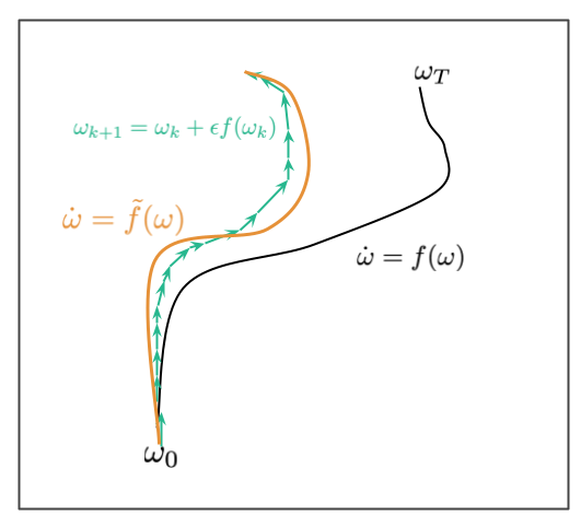
Let's say we have a differential equation $\dot{\omega} = f(\omega)$. The solution to this ODE with initial condition $\omega_0$ is a continuous trajectory $\omega_t$, shown in the image in black. We usually can't compute this solution in closed form, and instead simulate the ODE using the Euler's method, $\omega_{k+1} = \omega_k + \epsilon f(\omega_k)$. This results in a discrete trajectory shown in teal. Due to discretization error, for finite stepsize $\epsilon$, this discrete path may not lie exactly where the continuous black path lies. Errors accumulate over time, as shown in this illustration. The goal of backward error analysis is to find a different ODE, $\dot{\omega} = \tilde{f}(\omega)$ such that the approximate discrete path we got from Euler's method lieas near the the continuous path which solves this new ODE. Our goal is to reverse engineer a modified $\tilde{f}$ such that the discrete iteration can be well-modelled by an ODE.

Why is this useful? Because the form $\tilde{f}$ takes can reveal interesting aspects of the behaviour of the discrete algorithm, particularly if it has any implicit bias towards moving into different areas of the space. When the authors apply this technique to (full-batch) gradient descent, it already suggests the kind of implicit regularization bias gradient descent has.

In Gradient descent with a cost function $C$, the original ODE is $f(\omega) = -\nabla C (\omega)$. The modified ODE which corresponds to a finite stepsize $\epsilon$ takes the form $\dot{\omega} = -\nabla\tilde{C}_{GD}(\omega)$ where

$$
\tilde{C}_{GD}(\omega) = C(\omega) + \frac{\epsilon}{4} \|\nabla C(\omega)\|^2
$$

So, gradient descent with finite stepsize $\epsilon$ is like running gradient flow, but with an added penalty that penalises the gradients of the loss function. The second term is what Barret and Dherin (2021) call  implicit gradient regularization.

Stochastic Gradients

Analysing SGD in this framework is a bit more difficult because the trajectory in stochastic gradient descent is, well, stochastic. Therefore, you don't have have a single discrete trajectory to optimize, but instead you have a distribution of different trajectories which you'd traverse if you randomly reshuffle your data. Here's a picture illustrating this situation:

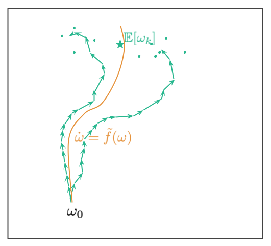
Starting from the initial point $\omega_0$ we now have multiple trajectories. These correspond to different ways we can shuffle data (in the paper we assume we have a fixed allocation of datapoints to minibatches, and the randomness comes from the order in which the minibatches are considered). The two teal trajectories illustrate two potential paths. The paths end up at a random location, the teal dots show additional random endpoints where trajectories may end up at. The teal star shows the mean of the distribution of random trajectory endpoints.

The goal in (Smith et al, 2021) is to reverse-engineer an ODE so that the continuous (orange) path lies close to this mean location. The corresponding ODE is of the form $\dot{omega} = -\nabla C_{SGD}(\omega)$, where

$$
\tilde{C}_{SGD}(\omega) = C(\omega) + \frac{\epsilon}{4m} \sum_{k=1}^{m} \|\nabla \hat{C}_k(\omega)\|^2,
$$

where $\hat{C}_k$ is the loss function on the $k^{th}$ minibatch. There are $m$ minibatches in total. Note that this is similar to what we had for gradient descent, but instead of the norm of the full-batch gradient we now have the average norm of minibatch gradients as the implicit regularizer. Another interesting view on this is to look at the difference between the GD and SGD regularizers:

$$
\tilde{C}_{SGD} = \tilde{C}_{GD} + \frac{\epsilon}{4m} \sum_{k=1}^{m} \|\nabla \hat{C}_k(\omega) - C(\omega)\|^2
$$

This additional regularization term, $\frac{1}{m}\sum_{k=1}^{m} \|\nabla \hat{C}_k(\omega) - C(\omega)\|^2$, is something like the total variance of minibatch gradients (the trace of the empirical Fisher information matrix). Intuitively, this regularizer term will avoid parts of the parameter-space where the variance of gradients calculated over different minibatches is high.

Importantly, while $C_{GD}$ has the same minima as $C$, this is no longer true for $C_{SGD}$. Some minima of $C$ where the variance of gradients is high, is no longer a minimum of $C_{SGD}$. As an implication, not only does SGD follow different trajectories than full-batch GD, it may also converge to completely different solutions.

As a sidenote, there are many versions of SGD, based on how data is sampled for the gradient updates. Here, it is assumed that the datapoints are assigned to minibatches, but then the minibatches are randomly sampled. This is different from randomly sampling datapoints with replacement from the training data (Li et al (2015) consider that case), and indeed an analysis of that variant may well lead to different results.

Connection to generalization

Why would an implicit regularization effect avoiding high minibatch gradient variance be useful for generalisation? Well, let's consider a cartoon illustration of two local minima below:

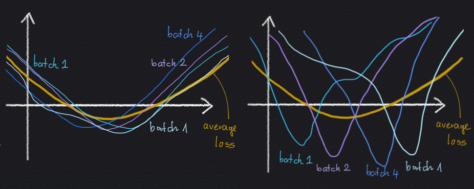
Both minima are the same as much as the average loss $C$ is concerned: the value of the minimum is the same, and the width of the two minima are the same. Yet, in the left-hand situation, the wide minimum arises as the average of several minibatch losses, which all look the same, and which all are relatively wide themselves. In the right-hand minimum, the wide average loss minimum arises as the average of a lot of sharp minibatch losses, which all disagree on where exactly the location of the minimum is.

If we have these two options, it is reasonable to expect the left-hand minimum to generalise better, because the loss function seems to be less sensitive to whichever specific minibatch we are evaluating it on. As a consequence, the loss function also may be less sensitive to whether a datapoint is in the training set or in the test set.

Summary

In summary, this paper is a very interesting analysis of stochastic gradient descent. While it has its limitations (which the authors don't try to hide and discuss transparently in the paper), it nevertheless contributes a very interesting new technique for analysing optimization algorithms with finite stepsize. I found the paper to be well-written, with the explanation of somewhat tedious details of the analysis clearly laid out. But perhaps I liked this paper most because it confirmed my intuitions about why SGD works, and what type of minima it tends to prefer.