Some Intuition on the Neural Tangent Kernel
Neural tangent kernels are a useful tool for understanding neural network training and implicit regularization in gradient descent. But it's not the easiest concept to wrap your head around. The paper that I found to have been most useful for me to develop an understanding is this one:
In this post I will illustrate the concept of neural tangent kernels through a simple 1D regression example. Please feel free to peruse the google colab notebook I used to make these plots.
Example 1: Warming up
Let's start from a very boring case begin with. Let's say we have a function defined over integers between -10 and 20. We parametrize our function as a look-up table, that is the value of the function $f(i)$ at each integer $i$ is described by a separate parameter $\theta_i = f(i)$. I'm initializing the parameters of this function as $\theta_i = 3i+2$. The function is shown by the black dots below:
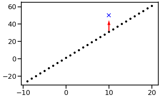
Now, let's consider what happens if we observe a new datapoint, $(x, y) =(10, 50)$, shown by the blue cross. We're going to take a gradient descent step updating $\theta$. Let's say we use the squared error loss function $(f(10; \theta) - 50)^2$ and a learning rate $\eta=0.1$. Because the function's value at $x=10$ only depends on one of the parameter $\theta_10$, only this parameter will be updated. The rest of the parameters, and therefore the rest of the function values remain unchanged. The red arrows illustrate the way function values move in a single gradient descent step: Most values don't move at all, only one of them moves closer to the observed data. Hence only one visible red arrow.
However, in machine learning we rarely parametrize functions as lookup tables of individual function values. This parametrization is pretty useless as it doesn't allow you to interpolate let alone extrapolate to unseen data. Let's see what happens in a more familiar model: linear regression.
Example 2: Linear function
Let's now consider the linear function $f(x, \theta) = \theta_1 x + \theta_2$. I initialize the parameters to $\theta_1=3$ and $\theta_2=1$, so at initialisation, I have exactly the same function over integers as I had in the first example. Let's look at what happens to this function as I update $\theta$ by performing single gradient descent step incorporating the observation $(x, y) =(10, 50)$ as before. Again, red arrows are show how function values move:
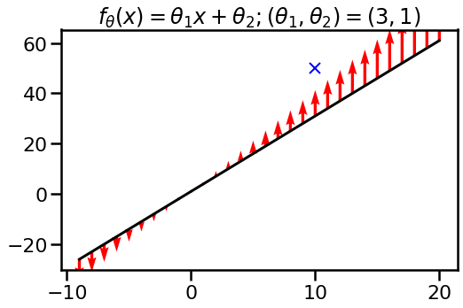
Whoa! What's going on now? Since individual function values are no longer independently parametrized, we can't move them independently. The model binds them together through its global parameters $\theta_1$ and $\theta_2$. If we want to move the function closer to the desired output $y=50$ at location $x=10$ the function values elsewhere have to change, too.
In this case, updating the function with an observation at $x=10$ changes the function value far away from the observation. It even changes the function value in the opposite direction than what one would expect.. This might seem a bit weird, but that's really how linear models work.
Now we have a little bit of background to start talking about this neural tangent kernel thing.
Meet the neural tangent kernel
Given a function $f_\theta(x)$ which is parametrized by $\theta$, its neural tangent kernel $k_\theta(x, x')$ quantifies how much the function's value at $x$ changes as we take an infinitesimally small gradient step in $\theta$ incorporating a new observation at $x'$. Another way of phrasing this is: $k(x, x')$ measures how sensitive the function value at $x$ is to prediction errors at $x'$.
In the plots before, the size of the red arrows at each location $x$ were given by the following equation:
$$
\eta \tilde{k}_\theta(x, x') = f\left(x, \theta + \eta \frac{f_\theta(x')}{d\theta}\right) - f(x, \theta)
$$
In neural network parlance, this is what's going on: The loss function tells me to increase the function value $f_\theta(x')$. I back-propagate this through the network to see what change in $\theta$ do I have to make to achieve this. However, moving $f_\theta(x')$ this way also simultaneously moves $f_\theta(x)$ at other locations $x \neq x'$. $\tilde{k}_\theta(x, x')$ expresses by how much.
The neural kernel is basically something like the limit of $\tilde{k}$ in as the stepsize becomes infinitesimally small. In particular:
$$
k(x, x') = \lim_{\eta \rightarrow 0} \frac{f\left(x, \theta + \eta \frac{df_\theta(x')}{d\theta}\right) - f(x, \theta)}{\eta}
$$
Using a 1st order Taylor expansion of $f_\theta(x)$, it is possible to show that
$$
k_\theta(x, x') = \left\langle \frac{df_\theta(x)}{d\theta} , \frac{f_\theta(x')}{d\theta} \right\rangle
$$
As homework for you: find $k(x, x')$ and/or $\tilde{k}(x, x')$ for a fixed $\eta$ in the linear model in the pervious example. Is it linear? Is it something else?
Note that this is a different derivation from what's in the paper (which starts from continuous differential equation version of gradient descent).
Now, I'll go back to the examples to illustrate two more important property of this kernel: sensitivity to parametrization, and changes during training.
Example 3: Reparametrized linear model
It's well known that neural networks can be repararmetized in ways that don't change the actual output of the function, but which may lead to differences in how optimization works. Batchnorm is a well-known example of this. Can we see the effect of reparametrization in the neural tangent kernel? Yes we can. Let's look at what happens if I reparametrize the linear function I used in the second example as:
$$
f_\theta(x) = \theta_1 x + \color{blue}{10\cdot}\theta_2
$$
but now with parameters $\theta_1=3, \theta_2=\color{blue}{0.1}$. I highlighted in blue what changed. The function itself, at initialization is the same since $10 * 0.1 = 1$. The function class is the same, too, as I can still implement arbitrary linear functions. However, when we look at the effect of a single gradient step, we see that the function changes differently when gradient descent is performed in this parametrisation.
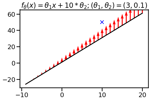
In this parametization, it became easier for gradient descent to push the whole function up by a constant, while in the previous parametrisation it decided to change the slope. What this demonstrates is that the neural tangent kernel $k_\theta(x, x')$ is sensitive to reparametrization.
Example 4: tiny radial basis function network
While the linear models may be good illustration, let's look at what $k_\theta(x, x')$ looks like in a nonlinear model. Here, I'll consider a model with two squared exponential basis functions:
$$
f_\theta(x) = \theta_1 \exp\left(-\frac{(x - \theta_2)^2}{30}\right) + \theta_3 \exp\left(-\frac{(x - \theta_4)^2}{30}\right) + \theta_5,
$$
with initial parameter values $(\theta_1, \theta_2, \theta_3, \theta_4, \theta_5) = (4.0, -10.0, 25.0, 10.0, 50.0)$. These are chosen somewhat arbitrarily and to make the result visually appealing:
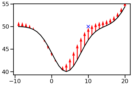
We can visualise the function $\tilde{k}_\theta(x, 10)$ directly, rather than plotting it on top the function. Here I also normalize it by dividing by $\tilde{k}_\theta(10, 10)$.
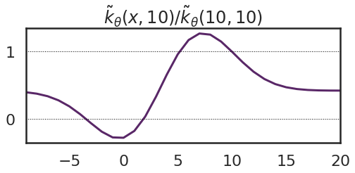
What we can see is that this starts to look a bit like a kernel function in that it has higher values near $10$ and decreases as you go farther away. However, a few things are worth noting: the maximum of this kernel function is not at $x=1o$, but at $x=7$. It means, that the function value $f(7)$ changes more in reaction to an observation at $x'=10$ than the value $f(10)$. Secondly, there are some negative values. In this case the previous figure provides a visual explanation why: we can increase the function value at $x=10$ by pushing the valley centred at $\theta_1=4$ away from it, to the left. This parameter change in turn decreases function values on the left-hand wall of the valley. Third, the kernel function converges to a positive constant at its tails - this is because of the offset $\theta_5$.
Example 5: Changes as we train
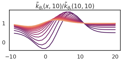
Now I'm going to illustrate another important property of the neural tangent kernel: in general, the kernel depends on the parameter value $\theta$, and therefore it changes as the model is trained. Here I show what happens to the kernel as I take 15 gradient ascent steps trying to increase $f(10)$. The purple curve is the one I had at initialization (above), and the orange ones show the kernel at the last gradient step.
The corresponding changes to the function $f_\theta_t$ changes are shown below:
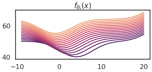
So we can see that as the parameter changes, the kernel also changes. The kernel becomes flatter. An explanation of this is that eventually we reach a region of parameter space, where $\theta_4$ changes the fastest.
Why is this interesting?
It turns out the neural tangent kernel becomes particularly useful when studying learning dynamics in infinitely wide feed-forward neural networks. Why? Because in this limit, two things happen:
- First: if we initialize $\theta_0$ randomly from appropiately chosen distributions, the initial NTK of the network $k_{\theta_0}$ approaches a deterministic kernel as the width increases. This means, that at initialization, $k_{\theta_0}$ doesn't really depend on $\theta_0$ but is a fixed kernel independent of the specific initialization.
- Second: in the infinite limit the kernel $k_{\theta_t}$ stays constant over time as we optimise $\theta_t$. This removes the parameter dependence during training.
These two facts put together imply that gradient descent in the infinitely wide and infinitesimally small learning rate limit can be understood as a pretty simple algorithm called kernel gradient descent with a fixed kernel function that depends only on the architecture (number of layers, activations, etc).
These results, taken together with an older known result by Neal, (1994), allows us to characterise the probability distribution of minima that gradient descent converges to in this infinite limit as a Gaussian process. For details, see the paper mentioned above.
Don't mix your kernels
There are two somewhat related sets of results both involving infinitely wide neural netwoks and kernel functions, so I just wanted to clarify the difference between them:
- the older, well-known result by Neal, (1994), later extended by others, is that the distribution of $f_\theta$ under random initialization of $\theta$ converges to a Gaussian process. This Gaussian process has a kernel or covariance function which is not, in general, the same as the neural tangent kernel. This old result doesn't say anything about gradient descent, and is typically used to motivate the use of Gaussian process-based Bayesian methods.
- the new, NTK, result is that the evolution of $f_{\theta_t}$ during gradient descent training can be described in terms of a kernel, the neural tangent kernel, and that in the infinite limit this kernel stays constant during training and is deterministic at initialization. Using this result, it is possible to show that in some cases the distribution of $f_{\theta_t}$ is a Gaussian process at every timestep $t$, not just at initialization. This result also allows us to identify the Gaussian process which describes the limit as $t \rightarrow \infty$. This limiting Gaussian process however is not the same as the posterior Gaussian process which Neal and others would calculate on the basis of the first result.
So I hope this post helps a bit by building some intuition about what the neural tangent kernel is. If you're interested, check out the simple colab notebook I used for these illustrations.