Causal Inference 3: Counterfactuals
Counterfactuals are weird. I wasn't going to talk about them in my MLSS lectures on Causal Inference, mainly because wasn't sure I fully understood what they were all about, let alone knowing how to explain it to others. But during the Causality Panel, David Blei made comments about about how weird counterfactuals are: how difficult they are to explain and wrap one's head around. So after that panel discussion, and with a grand total of 5 slides finished for my lecture on Thursday, I said "challenge accepted". The figures and story I'm sharing below are what I came up with after that panel discussion as I finally understood how to think about counterfactuals. I'm hoping others will find them illuminating, too.
This is the third in a series of tutorial posts on causal inference. If you're new to causal inferenece, I recommend you start from the earlier posts:
- Part 1: Intro to causal inference and do-calculus
- Part 2: Illustrating Interventions with a Toy Example
- ➡️️ Part 3: Counterfactuals
- Part 4: Causal Diagrams, Markov Factorization, Structural Equation Models
Counterfactuals
Let me first point out that counterfactual is one of those overloaded words. You can use it, like Judea Pearl, to talk about a very specific definition of counterfactuals: a probablilistic answer to a "what would have happened if" question (I will give concrete examples below). Others use the terms like counterfactual machine learning or counterfactual reasoning more liberally to refer to broad sets of techniques that have anything to do with causal analysis. In this post, I am going to focus on the narrow Pearlian definition of counterfactuals. As promised, I will start with a few examples:
Example 1: David Blei's election example
This is an example David brought up during the Causality Panel and I referred back to this in my talk. I'm including it here for the benefit of those who attended my MLSS talk:
Given that Hilary Clinton did not win the 2016 presidential election, and given that she did not visit Michigan 3 days before the election, and given everything else we know about the circumstances of the election, what can we say about the probability of Hilary Clinton winning the election, had she visited Michigan 3 days before the election?
Let's try to unpack this. We are are interested in the probability that:
- she hypothetically wins the election
conditionied on four sets of things:
- she lost the election
- she did not visit Michigan
- any other relevant an observable facts
- she hypothetically visits Michigan
It's a weird beast: you're simultaneously conditioning on her visiting Michigan and not visiting Michigan. And you're interested in the probability of her winning the election given that she did not. WHAT?
Why would quantifying this probability be useful? Mainly for credit assignment. We want to know why she lost the election, and to what degree the loss can be attributed to her failure to visit Michigan three days before the election. Quantifying this is useful, it can help political advisors make better decisions next time.
Example 2: Counterfactual fairness
Here's a real-world application of counterfactuals: evalueting the efairness of individual decisions. Consider this counterfactual question:
Given that Alice did not get promoted in her job, and given that she is a woman, and given everything else we can observe about her circumstances and performance, what is the probability of her getting a promotion if she was a man instead?
Again, the main reason for asking this question is to establish to what degree being a woman is directly responsible for the observed outcome. Note that this is an individual notion of fairness, unlike the aggregate assessment of whether the promotion process is fair or unfair statistically speaking. It may be that the promotion system is pretty fair overall, but in the particular case of Alice unfair discrimination took place.
A counterfactual question is about a specific datapoint, in this case Alice.
Another weird thing to note about this counterfactual is that the intervention (Alice's gender magically changing to male) is not something we could ever implement or experiment with in practice.
Example 3: My beard and my PhD
Here's the example I used in my talk, and will use throughout this post: I want to understand to what degree having a beard contributed to getting a PhD:
Given that I have a beard, and that I have a PhD degree, and everything else we know about me, with what probability would I have obtained a PhD degree, had I never grown a beard.
Before I start describing how to express this as a probability, let's first think about what we intuitively expect the answer to be? In the grand scheme of things, my beard probably was not a major contributing factor to getting a PhD. I would have pursued PhD studies, and probably completed my degree, even if something would have prevented me to keep my beard. So
We expect the answer to this counterfactual to be a high probability, something close to 1.
Observational queries
Let's start with the simplest thing one can do to attempt to answer my counterfactual question: collect some data about individuals, whether they have beards, whether they have PhDs, whether they are married, whether they are fit, etc. Here's a cartoon illustration of such dataset:
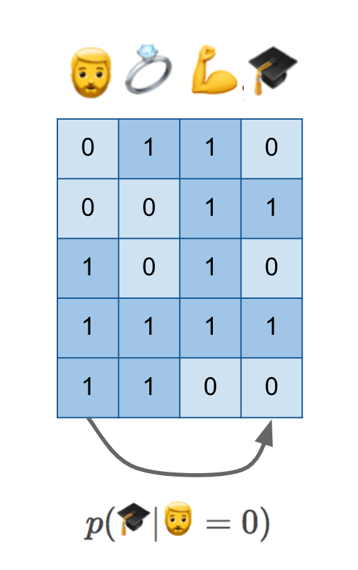
I am in this dataset, or someone just like me is in the dataset, in row number four: I have a beard, I am married, I am obviously very fit (this was the point where I hoped the audience would get the joke and laugh, and thankfully they did), and I have a PhD degree. I have it all.
If we have this data and do normal statistical machine learning, without causal reasoning, we'd probably attempt to estimate $p(🎓\vert 🧔=0)$, the conditional probability of possessing a PhD degree given the absence of a beard. As I show at the bottom, this is like predicting values in one column from values in another column.
You hopefully know enough about causal inference by now to know that $p(🎓\vert 🧔=0)$ is certainly not the quantity we seek. Without additional knowledge of causal structure, it can't generalize to hypothetical scenarios and interventions we care about her. There might be hidden confounders. Perhaps scoring high on the autism spectrum makes it more likely that you grow a beard, and it may also makes it more likely to obtain a PhD. This conditional isn't aware if the two quantities are causally related or not.
Intervention queries
We've learned in the previous two posts that if we want to reason about interventions, we have to express a different conditional distribution, $p(🎓\vert do(🧔=0))$. We also know that in order to reason about this distribution, we need more than just a dataset, we also need a causal diagram. Let's add a few things to our figure:
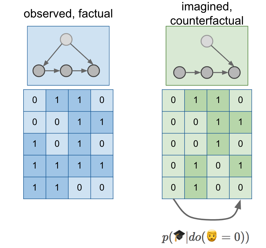
Here, I drew a cartoon causal diagram on top of the data just for illustration, it was simply copy-pasted from previous figures, and does not represent a grand unifying theory of beards and PhD degrees. But let's assume our causal diagram describes reality.
The causal diagram lets us reason about the distribution of data in an alternative world, a parallel universe if you like, in which everyone is somehow magically prevented to grow a beard. You can imagine sampling a dataset from this distribution, shown in the green table. We can measure the association between PhD degrees and beards in this green distribution, which is precisely what $p(🎓\vert do(🧔=0))$ means. As shown by the arrow below the tables, $p(🎓\vert do(🧔=0))$ is about predicting columns of the green dataset from other columns of the green dataset.
Can $p(🎓\vert do(🧔=0))$ express the counterfactual probability we seek? Well, remember that we expected that I would have obtained a PhD degree with a high probability even without a beard. However, $p(🎓\vert do(🧔=0))$ talks about a the PhD of a random individual after a no-beard intervention. If you take a random person off the street, shave their beard if they have one, it is not very likely that your intervention will cause them to get a PhD with a high probability. Not to mention that your intervention has no effect on most women and men without beards. We intuitively expect $p(🎓\vert do(🧔=0))$ to be close to the base-rate of PhD degrees $p(🎓)$, which is apparently somewhere around 1-3%.
$p(🎓\vert do(🧔=0))$ talks about a randomly sampled individual, while a counterfactual talks about a specific individual
Counterfactuals are "personalized" in the sense that you'd expect the answer to change if you substitute a different person in there. My father has a mustache, (let's classify that as a type of beard for pedagogical purposes), but he does not have a PhD degree. I expect that preventing him to grow a mustache would not have made him any more likely to obtain a PhD. So his counterfactual probability would be a probability close to 0.
The counterfactual probabilities vary from person to person. If you calculate them for random individuals, and average the probabilities, you should expect to to get something like $p(🎓\vert do(🧔=0))$ in expectation. (More on this connection later.) But we not interested in the population mean now, but are interested in calculating the probabilities for each individual.
Counterfactual queries
To finally explain counterfactuals, I have to step beyond causal graphs and introduce another concept: structural equation models.
Structural Equation Models
A causal graph encodes which variables have a direct causal effect on any given node - we call these causal parents of the node. A structural equation model goes one step further to specify this dependence more explicitly: for each variable it has a function which describes the precise relationship between the value of each node the value of its causal parents.
It's easiest to illustrate this through an example: here's a causal graph of an online advertising system, taken from the excellent paper of Bottou et al, (2013):
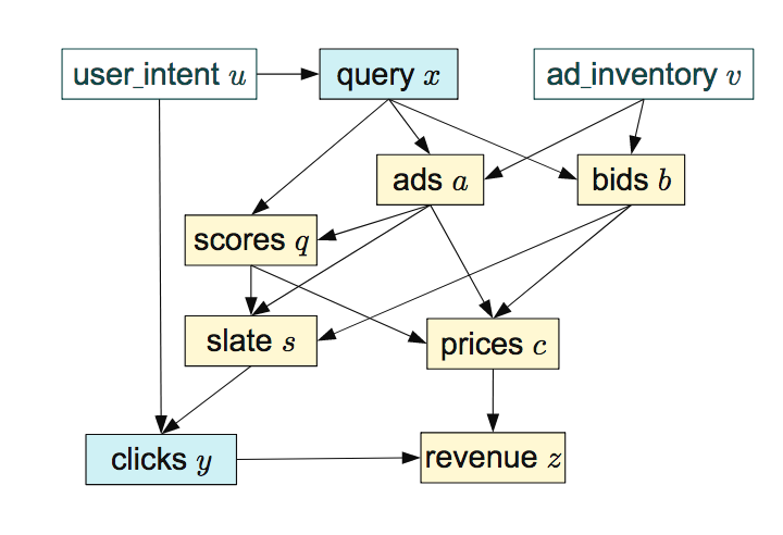
It doesn't really matter what these variables mean, if interested, read the paper. The dependencies shown by the diagram are equivalently encoded by the following set of equations:
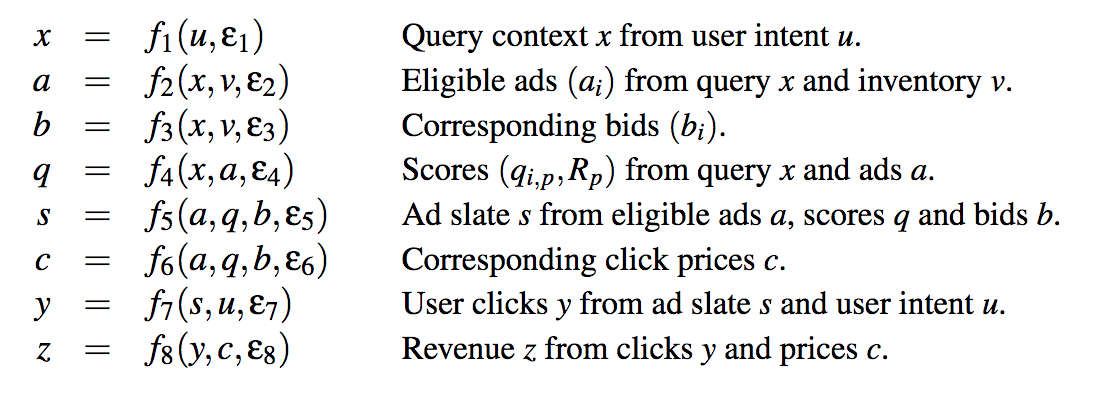
For each node in the graph above we now have a corresponding function $f_i$. The arguments of each function are the causal parents of the variable it instantiates, e.g. $f_1$ computes $x$ from its causal parent $u$, and $f_2$ computes $a$ from its causal parents $x$ and $v$. In order to allow for nondeterministic relationship between the variables, we additionally allow each function $f_i$ to take another input, $\epsilon_i$ which you can think of as a random number. Through the random input $\epsilon_1$, the output of $f_1$ can be random given a fixed value of $u$, hence giving rise to a conditional distribution $p(x \vert u)$.
The structural equation model (SEM) entails the causal graph, in that you can reconstruct the causal graph by looking at the inputs of each function. It also entails the joint distribution, in that you can "sample" from an SEM by evaluating the functions in order, plugging in the random $\epsilon$s where needed.
In a SEM an intervention on a variable, say $q$, can be modelled by deleting the corresponding function, $f_4$, and replacing it with another function. For example $do(Q = q_0)$ would correspond to a simple assignment to a constant $\tilde{f}_4(x, a) = q_0$.
Back to the beard example
Now that we know what SEMs are we can return to our example of beards and degrees. Let's add a few more things to the figure:
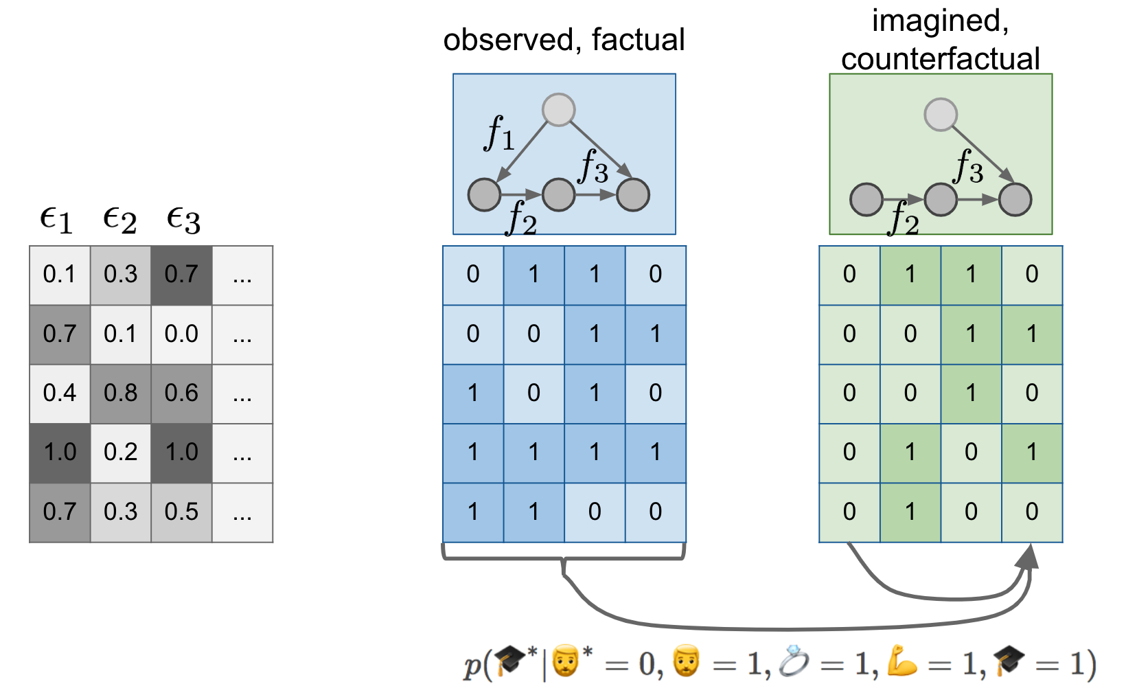
First change is, that instead of just a causal graph, I now assume that we model the world by a fully specified structural equation model. I signify this lazily by labelling the causal graph with the functions $f_1, f_2, f_3$ over the graph. Notice that the SEM of the green situation is the same as the SEM in the blue case, except that I deleted $f_1$ and replaced it with a constant assignment. But $f_2$ and $f_3$ are the same between the blue and the green models.
Secondly, I make the existence of the $\epsilon_i$ noise variables explicit, and show their values (it's all made up of course) in the gray table. If you feed the first row of epsilons to the blue structural equation model, you get the first blue datapoint $0110$. If you feed the same epsilons to the green SEM, you get the first green datapoint $(0110)$. If you feed the second row of epsilons to the models, you get the second rows in the blue and green tables, and so on...
I like to think about the first green datapoint as the parallel twin of the first blue datapoint. To talk about interventions I talked about this making predictions about a parallel universe where nobody has a beard. Now imagine that for every person who lives in our observable universe, there is a corresponding person, their parallel twin, in this parallel universe. Your twin is same in every respect as you, except for the absence of any beard you might have and any downstream consequences of having a beard. If you don't have a beard in this universe, your twin is an exact copy of you in every respect. Indeed, notice that the first blue datapoint is the same as the first green datapoint in my example.
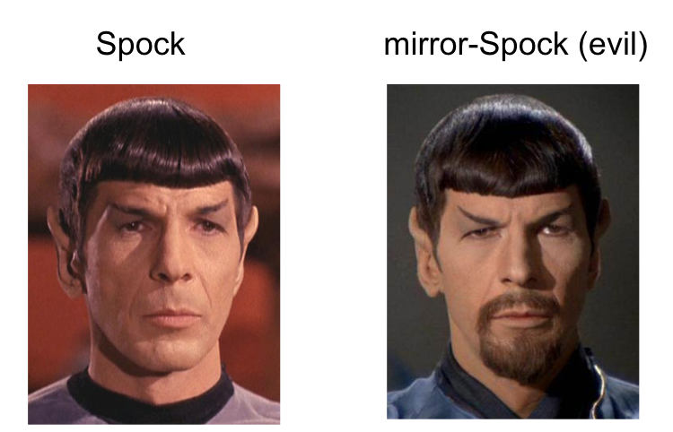
You may know I'm a Star Trek fan and I like to use Star Trek analogies to explain things: In Star Trek, there is this concept called the mirror universe. It's a parallel universe populated by the same people who live in the normal universe, except that everyone who is good in the real universe is evil in the mirror universe. Hilariously, the mirror version of Spock, one of the main protagonists, has a goatie in this mirror universe. This is how you could tell if you're looking at evil mirror-Spock or normal Spock when watching the episode. This explains, sadly, why I'm using beards to explain counterfactuals. Here are Spock and mirror-Spock:
Now that we established the twin datapoint metaphor, we can say that counterfactuals are
making a prediction about features of the unobserved twin datapoint based on features of the observed datapoint.
Crucially, this was possible because we used the same $\epsilon$s in both the blue and the green SEM. This induces a joint distribution between variables in the observable regime, and variables in the unobserved, counterfactual regime. Columns of the green table are no longer independent of columns of the blue table. You can start predicting values in the green table using values in the blue table, as illustrated by the arrows below them.
Mathematically, a counterfactual is the following conditional probability:
$$
p(🎓^\ast \vert 🧔^\ast = 0, 🧔=1, 💍=1, 💪=1, 🎓=1),
$$
where variables with an $^\ast$ are unobserved (and unobservable) variables that live in the counterfactual world, while variables without $^\ast$ are observable.
Looking at the data, it turns out that mirror-Ferenc, who does not have a beard, is married and has PhD, but is not quite as strong as observable Ferenc.
Another way to draw this
Here is another drawing that some of you might find more appealing, especially those who are are into GANs, VAEs and similar generative models:
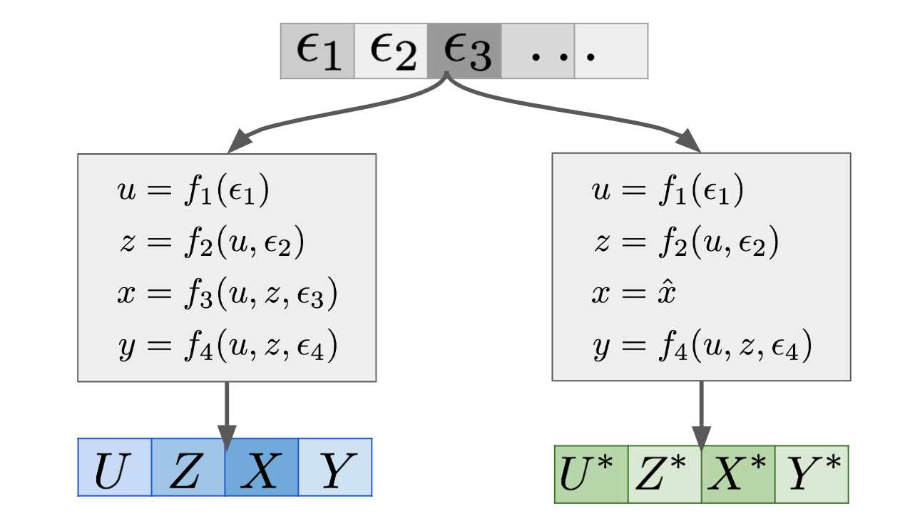
A SEM is essentially a generative model of data, which uses some noise variables $\epsilon_1, \epsilon_2, \ldots$ and turns them into observations $(U,Z,X,Y)$ in this example. This is shown in the left-hand branch of the graph above. Now if you want to make counterfactual statements under the intervention $X=\hat{x}$, you can construct a mutilated SEM, which is the same SEM except with $f_3$ deleted and replaced with the constant assignment $x = \hat{x}$. This modified SEM is shown in the right-hand branch. If you feed the $\epsilon$s into the mutilated SEM, you get another set of variables $(U^\ast,Z^\ast,X^\ast,Y^\ast)$, shown in green. These are the features of the twin as it were. This joint generative model over $(U,Z,X,Y)$ and $(U^\ast,Z^\ast,X^\ast,Y^\ast)$ defines a joint distribution over the combined set of variables $(U,Z,X,Y,U^\ast,Z^\ast,X^\ast,Y^\ast)$. Therefore, now you can calculate all sorts of conditionals and marginals of this joint.
Of particular interest are these conditionals:
$$
p(y^\ast \vert X^\ast = \hat{x}, X = x, Y = y, U = u, Z = z),
$$
which is a counterfactual prediction. In reality, since $X^\ast = \hat{x}$ holds with a probability of $1$, we can drop that conditioning.
My notation here is a bit sloppy, there are a lot of things going on implicitly under the hood, which I'm not making explicit in the notation. I'm sorry if it causes any irritation to people, I want to avoid overcomplicating things at this point. Now is a good time to point out that Pearl's notation, including do-notation is often criticized, but people use it because now it's widely adopted.
We can also express the intervention conditional $p(y\vert do(x))$ using this (somewhat sloppy) notation as:
$$
p(y\vert do(X=\hat{x})) = p(y^\ast \vert X^\ast = \hat{x})
$$
We can see that the intervention conditional only contains variables with an $^\ast$ so it does not require the joint distribution of $(U,Z,X,Y,U^\ast,Z^\ast,X^\ast,Y^\ast)$ only the marginal of the $^\ast$ variables $(X^\ast, Z^\ast,X^\ast,Y^\ast)$. As a consequence in order to talk about $p(y\vert do(X=\hat{x}))$ we did not need to introduce SEMs or talk about the epsilons.
Furthermore, notice the following equality:
\begin{align}
p(y\vert do(X=\hat{x})) &= p(y^\ast \vert X^\ast = \hat{x}) \\
&= \int_{x,y,u,z} p(y^\ast \vert X^\ast = \hat{x}, X = x, Y = y, U = u, Z = z) p(x,y,u,z) dx dy du dz \\
&= \mathbb{E}_{p_{X,Y,U,Z}} p(y^\ast \vert X^\ast = \hat{x}, X = x, Y = y, U = u, Z = z),
\end{align}
in other words, the intervention conditional $p(y\vert do(X=\hat{x}))$ is the average of counterfactuals over the obserevable population. This was something that I did did not realize before my MLSS tutorial, and it was pointed out to me by a student in the form of a question. In hindsight, of course this is true!
Summary
God, this was a loooong post. If you're still reading, thanks, I hope it was useful. I wanted to close with a few slightly philosophical remarks on counterfactuals.
Counterfactuals are often said to be unscientific, primarily because they are not empirically testable. In normal ML we are used to benchmark datasets, and that the quality of our predictions can always be tested on some test dataset. In causal ML, not everything can be directly tested or empirically benchmarked. For interventions, the best test is to run a randomized controlled trial to directly measure $p(y\vert do(X=x))$ if you can, and then use this experiemental data to evaluate your causal inferences. But some interventions are impossible to carry out in practice. Think about all the work on fairness reasoning about interventions on gender or race. So what to do then?
In the world of counterfactuals this is an even bigger problem, as it is outright impossible to observe the variables you make predictions about. You can't go back in time and rerun history with exactly the same circumstances except for a tiny change. You can't travel to parallel universes (at least not before the 24th century, according to Star Trek). Counterfactual judgments remain hypothetical, subjective, untestable, unfalsifiable. There can be no MNIST or Imagenet for counterfactuals that satisfies everyone, though some good datasets exist, they are for specific scenarios where explicit testing is possible (e.g. offline A/B testing), or make use of simulators instead of "real" data.
Despite it being untestable, and difficult to interpret, humans make use of counterfactual statements all the time, and intuitively it feels like they are pretty useful for intelligent behaviour. Being able to pinpoint the causes that lead to a particular situation or outcome is certainly useful for learning, reasoning and intelligence. So my strategy for now is to ignore the philosophical debate about counterfactuals, and just get on with it, knowing that the tools are there if such predictions have to be made.