Causal inference 4: Causal Diagrams, Markov Factorization, Structural Equation Models

This post is written with my PhD student and now guest author Patrik Reizinger and is part 4 of a series of posts on causal inference:

• Part 1: Intro to causal inference and do-calculus
• Part 2: Illustrating Interventions with a Toy Example
• Part 3: Counterfactuals
• ➡️️ Part 4: Causal Diagrams, Markov Factorization, Structural Equation Models

One way to think about causal inference is that causal models require a more fine-grained models of the world compared to statistical models. Many causal models are equivalent to the same statistical model, yet support different causal inferences. This post elaborates on this point, and makes the relationship between causal and statistical models more precise.

Markov factorization

Do you remember those combinatorics problems from school where the question was how many ways exist to get from a start position to a target field on a chessboard? And you can only move one step right or one step down. If you remember, then I need to admit that we will not consider problems like that. But its (one possible) takeaway actually can help us to understand Markov factorizations.

You know, it is totally indifferent how you traversed the chessboard, the result is the same. So we can say that - from the perspective of target position and the process of getting there - this is a many-to-one mapping. The same holds for random variables and causal generative models.

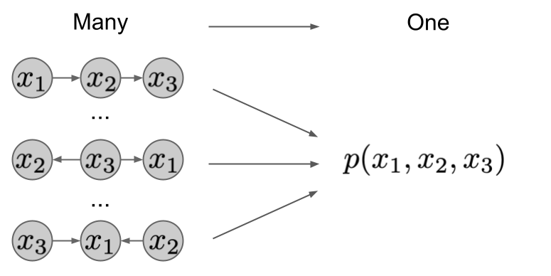
If you have a bunch of random variables - let's call them $X_1, X_2, \dots, X_n$ -, their joint distribution is $p \left(X_1, X_2, \dots, X_n \right) $. If you invoke the chain rule of probability, you will have several options to express this joint as a product of factors:

$$
p \left(X_1, X_2, \dots, X_n \right) = \prod p(X_{\pi_i}\vert X_{\pi_1}, \ldots, X_{\pi_{i-1}}),
$$

where $\pi_i$ is a permutation of indices. Since you can do this for any permutation $\pi$, the mapping between such factorizations and the joint distribution they express is many-to-one. As you can see this in the image below. The different factorizations induce a different graph, but have the same joint distribution.

Since you are reading this post, you may already be aware that in causal inference we often talk about a causal factorization, which looks like

$$
p \left(X_1, X_2, \dots, X_n \right) = \prod_{i=1}^{n} p\left(X_i | X_{\mathrm{pa}(i)}\right),
$$

where $\mathrm{pa}(X_i)$ denotes the causal parents of node $X_i$. This is one of many possible ways you can factorize the joint distribution, but we consider this one special. In the recent work, Schölkopf et al. call it a disentangled model. What are disentangled models? Disentangled factors describe independent aspects of the mechanism that generated the data. And they are not independent because you factored them in this way, but you were looking for this factorization because its factors are independent.

In other words, for every joint distribution there are many possible factorizations, but we assume that only one, the causal or disentangled factorization, describes the true underlying process that generated the data.

Let's consider an example for disentangled models. We want to model the joint distribution of altitude $A$ and temperature $T$. In this case, the causal direction is $A \rightarrow T$ - if the altitude changes, the distribution of the temperature will change too. But you cannot change the altitude by artificially heating a city - otherwise we all would enjoy views as in Miami; global warming is real but fortunately has no altitude-changing effect.
In the end, we get the factorization of $p(A)p(T|A)$. The important insights here are the answers to the question: What do we expect from these factors? The previously-mentioned Schölkopf et al. paper calls the main takeaway the Independent Causal Mechanisms (ICM) Principle, i.e.

By conditioning on the parents of any factor in the disentangled model, the factor will neither be able to give you further information about other factors nor is able to influence them.

In the above example, this means that if you consider different countries with their altitude distributions, you can still use the same $p(T|A),$ i.e., the factors generalize well. For no influence, the example holds straight above the ICM Principle. Furthermore, knowing any of the factors - e.g. $p(A)$ - won't tell anything about the other (no information). If you know which country you are in, so will have no clue about the climate (if you consulted the website of the corresponding weather agency, that's what I call cheating). In the other direction, despite being the top-of-class student in climate matters, you won't be able to tell the country if somebody says to you that here the altitude is 350 meters and the temperature is 7°C!

Statistical vs causal inference

We discussed Markov factorizations, as they help us understand the philosophical difference between statistical and causal inference. The beauty, and a source of confusion, is that one can use Markov factorizations in both paradigms.

However, while using Markov factorizations is optional for statistical inference, it is a must for causal inference.

So why would a statistical inference person use Markov factorizations? Because they make life easier in the sense that you do not need to worry about too high electricty costs. Namely, factorized models of data can be computationally much more efficient. Instead of modeling a joint distribution directly, which has a lot of parameters - in the case of $n$ binary variables, that is $2^n-1$ different values -, a factorized version can be pretty lightweight and parameter-efficient. If you are able to factorize the joint in a way that you have 8 factors with $n/8$ variables each, then you can describe your model with $8\times2^{n/8}-1$ parameters. If $n=16$, that is $65,535$ vs $31$. Similarly, representing your distibution in a factorized form gives rise to efficient, general-purpose message-passing algorithms, such as belief propagation or expectation propagation.

On the other hand, causal inference people really need this, otherwise, they are lost. Because without Markov factorizations, they cannot really formulate causal claims.

A causal practicioner uses Markov factorizations, because this way she is able to reason about interventions.

If you do not have the disentangled factorization, you cannot model the effect of interventions on the real mechanisms that make the system tick.

Connection to domain adaptation

In plain machine learning lingo, what you want to do is domain adaptation, that is, you want to draw conclusions about a distribution you did not observe (these are the interventional ones). The Markov factorization prescribes ways in which you expect the distribution to change - one factor at a time - and thus the set of distributions you want to be able to robustly generalise to or draw inferences about.

Do calculus

Do-caclculus, the topic of the first post in the series, can be relatively simply described using Markov factorizations. As you remember, $\mathrm{do}(X=x)$ means that we set the variable $X$ to the value $x$, meaning that the distribution of that variable $p(X)$ collapses to a point mass. We can model this intervention mathematically by replacing the factor $p( x \vert \mathrm{pa}(X))$ by a Dirac-delta $\delta_x$, resulting in the deletion of all incoming edges of the intervened factors in the graphical model. We then marginalise over $x$ to calculate the joint distribution of the remaining variables. For example, if we have two variables $x$ and $y$ we can write:

$$
p(y\vert do(X=x_0)) = \int p(x,y) \frac{\delta(x - x_0)}{p(x\vert y)} dx
$$

SEMs, Markov factorization, and the reparamtrization trick

If you've read the previous parts in this series, you'll know that Markov factorizations aren't the only tool we use in causal inference. For counterfactuals, we used structural equation models (SEMs). In this part we will illustrate the connection between these with a cheesy reference to the reparametrization trick used in VAEs among others.

But before that, let's recap SEMs. In this case, you define the relationship between the child node and its parents via a functional assignment. For node $X$ with parents $\mathrm{pa}(X)$ it has the form of

$$
X = f(\mathrm{pa}(X), \epsilon),
$$

with some noise $\epsilon.$ Here, you should read "=" in the sense of an assigment (like in Python), in mathematics, this should be ":=".
The above equation expresses the conditional probability $ p\left(X| \mathrm{pa}(X)\right)$ as a deterministic function of $X$ and some noise variable $\epsilon$. Wait a second..., isn't it the same thing what the reparametrization trick does? Yes it is.

So the SEM formulation (called the implicit distribution) is related via the reparametrization trick to the conditional probability of $X$ given its parents.

Classes of causal models

Thus, we can say that a SEM is a conditional distribution, and vica versa. Okay, but how do the sets of these constructs relate to each other?
If you have a SEM, then you can read off the conditional, which is unique. On the other hand, you can find more SEMs for the same conditional. Just as you can express a conditional distribution in multiple different ways using different reparametrizations, it is possible to express the same Markov factorization by multiple SEMs. Consider for example that if your distribution is $\mathcal{N}(\mu,\sigma),$ then multiplying it by -1 gives you the same distribution. In this sense, SEMs are a richer class of models than Markov factorizations, thus they allow us to make inferences (counterfactual) which we weren't able to express in the more coarse grained language of Markov Factorizations.

As we discussed above, a single joint distribution has multiple valid Markov factorizations, and the same Markov factorization can be expressed as different SEMs. We can think of joint distributions, Markov factorizations, and SEMs as increasingly fine-grained model classes: joint distributions $\subset$ Markov facorizations $\subset$ SEMs. The more aspects of the data generating process you model, the more elaborate the set of inferences you can make become. Thus, Joint distributions allow you to make predictions under no mechanism shift, Markov factorizations allow you to model interventions, SEMs allow you to make counterfactual statements.

The price you pay for more expressive models is that they also get generally much harder to estimate from data. In fact, some aspects of causal models are impossible to infer from i.i.d. observational data. Moreover, some counterfactual inferences are experimentally not verifiable.