
ML beyond Curve Fitting: An Intro to Causal Inference and do-Calculus
Since writing this post back in 2018, I have extended this to a 4-part series on causal inference:
- ➡️️ Part 1: Intro to causal inference and do-calculus
- Part 2: Illustrating Interventions with a Toy Example
- Part 3: Counterfactuals
- Part 4: Causal Diagrams, Markov Factorization, Structural Equation Models
You might have come across Judea Pearl's new book, and a related interview which was widely shared in my social bubble. In the interview, Pearl dismisses most of what we do in ML as curve fitting. While I believe that's an overstatement (conveniently ignores RL for example), it's a nice reminder that most productive debates are often triggered by controversial or outright arrogant comments. Calling machine learning alchemy was a great recent example. After reading the article, I decided to look into his famous do-calculus and the topic causal inference once again.
Again, because this happened to me semi-periodically. I first learned do-calculus in a (very unpopular but advanced) undergraduate course Bayesian networks. Since then, I have re-encountered it every 2-3 years in various contexts, but somehow it never really struck a chord. I always just thought "this stuff is difficult and/or impractical" and eventually forgot about it and moved on. I never realized how fundamental this stuff was, until now.
This time around, I think I fully grasped the significance of causal reasoning and I turned into a full-on believer. I know I'm late to the game but I almost think it's basic hygiene for people working with data and conditional probabilities to understand the basics of this toolkit, and I feel embarrassed for completely ignoring this throughout my career.
In this post I'll try to explain the basics, and convince you why you should think about this, too. If you work on deep learning, that's an even better reason to understand this. Pearl's comments may be unhelpful if interpreted as contrasting deep learning with causal inference. Rather, you should interpret it as highlighting causal inference as a huge, relatively underexplored, application of deep learning. Don't get discouraged by causal diagrams looking a lot like Bayesian networks (not a coincidence seeing they were both pioneered by Pearl) they don't compete with, they complement deep learning.
Basics
First of all, causal calculus differentiates between two types of conditional distributions one might want to estimate. tldr: in ML we usually estimate only one of them, but in some applications we should actually try to or have to estimate the other one.
To set things up, let's say we have i.i.d. data sampled from some joint $p(x,y,z,\ldots)$. Let's assume we have lots of data and the best tools (say, deep networks) to fully estimate this joint distribution, or any property, conditional or marginal distribution thereof. In other words, let's assume $p$ is known and tractable. Say we are ultimately interested in how variable $y$ behaves given $x$. At a high level, one can ask this question in two ways:
-
observational $p(y\vert x)$: What is the distribution of $Y$ given that I observe variable $X$ takes value $x$. This is what we usually estimate in supervised machine learning. It is a conditional distribution which can be calculated from $p(x,y,z,\ldots)$ as a ratio of two of its marginals. $p(y\vert x) = \frac{p(x,y)}{p(x)}$. We're all very familiar with this object and also know how to estimate this from data.
-
interventional $p(y\vert do(x))$: What is the distribution of $Y$ if I were to set the value of $X$ to $x$. This describes the distribution of $Y$ I would observe if I intervened in the data generating process by artificially forcing the variable $X$ to take value $x$, but otherwise simulating the rest of the variables according to the original process that generated the data. (note that the data generating procedure is NOT the same as the joint distribution $p(x,y,z,\ldots)$ and this is an important detail).
Aren't they the same thing?
No. $p(y\vert do(x))$ and $p(y\vert x)$ are not generally the same, and you can verify this with several simple thought experiments. Say, $Y$ is the pressure in my espresso machine's boiler which ranges roughly between $0$ and $1.1$ bar depending on how long it's been turned on. Let $X$ be the reading of the built-in barometer. Let's say we jointly observe X and Y at random times. Assuming the barometer functions properly $p(y|x)$ should be a unimodal distribution centered around $x$, with randomness due to measurement noise. However, $p(y|do(x))$ won't actually depend on the value of $x$ and is generally the same as $p(y)$, the marginal distribution of boiler pressure. This is because artificially setting my barometer to a value (say, by moving the needle) won't actually cause the pressure in the tank to go up or down.
In summary, $y$ and $x$ are correlated or statistically dependent and therefore seeing $x$ allows me to predict the value of $y$, but $y$ is not caused by $x$ so setting the value of $x$ won't effect the distribution of $y$. Hence, $p(y\vert x)$ and $p(y\vert do(x))$ behave very differently. This simple example is just the tip of the iceberg. The differences between interventional and observational conditionals can be a lot more nuanced and hard to characterize when there are lots of variables with complex interactions.
Which one do I want?
Depending on the application you want to solve, you should seek to estimate one of these conditionals. If your ultimate goal is diagnosis or forecasting (i.e. observing a naturally occurring $x$ and inferring the probable values of $y$) you want the observational conditional $p(y\vert x)$. This is what we already do in supervised learning, this is what Judea Pearl called curve fitting. This is all good for a range of important applications such as classification, image segmentation, super-resolution, voice transcription, machine translation, and many more.
In applications where you ultimately want to control or choose $x$ based on the conditional you estimated, you should seek to estimate $p(y\vert do(x))$ instead. For example, if $x$ is a medical treatment and $y$ is the outcome, you are not merely interested in observing a naturally occurring treatment $x$ and predicting the outcome, we want to proactively choose the treatment $x$ given our understanding of how it effects the outcome $y$. Similar situations occur in system identification, control and online recommender systems.
What exactly is $p(y\vert do(x))$?
This is perhaps the main concept I haven't grasped before. $p(y\vert do(x))$ is in fact a vanilla conditional distribution, but it's not computed based on $p(x,z,y,\ldots)$, but a different joint $p_{do(X=x)}(x,z,y,\ldots)$ instead. This $p_{do(X=x)}$ is the joint distribution of data which we would observe if we actually carried out the intervention in question. $p(y\vert do(x))$ is the conditional distribution we would learn from data collected in randomized controlled trials or A/B tests where the experimenter controls $x$. Note that actually carrying out the intervention or randomized trials may be impossible or at least impractical or unethical in many situations. You can't do an A/B test forcing half your subjects to smoke weed and the other half to smoke placebo to understand the effect on marijuana on their health. Even if you can't directly estimate $p(y\vert do(x))$ from randomized experiments, the object still exists. The main point of causal inference and do-calculus is:
If I cannot measure $p(y\vert do(x))$ directly in a randomized controlled trial, can I estimate it based on data I observed outside of a controlled experiment?
How are all these things related?
Let's start with a diagram that shows what's going on if we only care about $p(y\vert x)$, i.e. the simple supervised learning case:
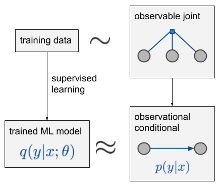
Let's say we observe 3 variables, $x, z, y$, in this order. Data is sampled i.i.d. from some observable joint distribution over 3 variables, denoted by the blue factor graph labelled 'observable joint'. If you don't know what a factor graph is, it's not important, the circles represent random variables, the little square represents a joint distribution of the variables it's connected to. We are interested in predicting $y$ from $x$, and say that $z$ is a third variable which we do not want to infer but we can also measure (I included this for completeness). The observational conditional $p(y\vert x)$ is calculated from this joint via simple conditioning. From the training data we can build a model $q(y\vert x;\theta)$ to approximate this conditional, for example using a deep net minimizing cross-entropy or whatever.
Now, what if we're actually interested in $p(y\vert do(x))$ rather than $p(y\vert x)$? This is what it looks like:
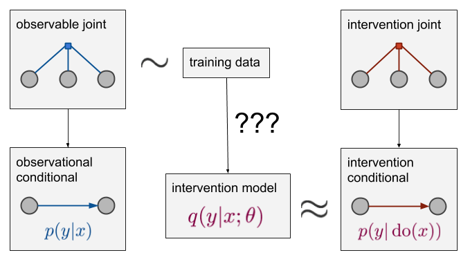
So, we still have the blue observed joint and data is still sampled from this joint. However, the object we wish to estimate is on the bottom right, the red intervention conditional $p(y\vert do(x))$. This is related to the intervention joint which is denoted by the red factor graph above it. It's a joint distribution over the same domain as $p$ but it's a different distribution. If we could sample from this red distribution (e.g. actually run a randomized controlled trial where we get to pick $x$), the problem would be solved by simple supervised learning. We could generate data from the red joint, and estimate a model directly from there. However, we assume this is not possible, and all we have is data sampled from the blue joint. We have to see if we can somehow estimate the red conditional $p(y\vert do(x))$ from the blue joint.
Causal models
If we want to establish a connection between the blue and the red joints, we must introduce additional assumptions about the causal structure of the data generating mechanism. The only way we can make predictions about how our distribution changes as a consequence of an interaction is if we know how the variables are causally related. This information about causal relationships is not captured in the joint distribution alone. We have to introduce something more expressive than that. Here is how what this looks like:
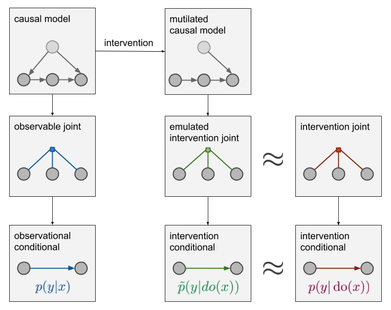
In addition to the observable joint we now also have a causal model of the world (top left) This causal model contains more detail than the joint distribution: it knows not only that pressure and barometer readings are dependent but also that pressure causes the barometer to go up and not the other way around. The arrows in this model correspond to the assumed direction of causation, and the absence of an arrow represents the absence of direct causal influence between variables. The mapping from causal diagrams to joint distributions is many-to-one: several causal diagrams are compatible with the same joint distribution. Thus, it is generally impossible to conclusively choose between different causal explanations by looking at observed data only.
Coming up with a causal model is a modeling step where we have to consider assumptions about how the world works, what causes what. Once we have a causal diagram, we can emulate the effect of intervention by mutilating the causal network: deleting all edges that lead into nodes in a $do$ operator. This is shown on the middle-top panel. The mutilated causal model then gives rise to a joint distribution denoted by the green factor graph. This joint has a corresponding conditional distribution $\tilde{p}(y\vert do(x))$, which we can use as our approximation of $p(y\vert do(x))$. If we got the causal structure qualitatively right (i.e. there are no missing nodes and we got the direction of arrows all correct), this approximation is exact and $\tilde{p}(y\vert do(x)) = p(y\vert do(x))$. If our causal assumptions are wrong, the approximation may be bogus.
Critically, to get to this green stuff, and thereby to establish the bridge between observational data and interventional distributions, we had to combine data with additional assumptions, prior knowledge if you wish. Data alone would not enable us to do this.
Do-calculus
Now the question is, how can we say anything about the green conditional when we only have data from the blue distribution. We are in a better situation than before as we have the causal model relating the two. To cut a long story short, this is what the so-called do-calculus is for. Do-calculus allows us to massage the green conditional distribution until we can express it in terms of various marginals, conditionals and expectations under the blue distribution. Do-calculus extends our toolkit of working with conditional probability distributions with four additional rules we can apply to conditional distributions with the $do$ operators in them. These rules take into account properties of the causal diagram. The details can't be compressed into a single blog post, but here is an introductory paper on them..
Ideally, as a result of a do-calculus derivation you end up with an equivalent formula for $\tilde{p}(y\vert do(x))$ which no longer has any do operators in them, so you estimate it from observational data alone. If this is the case we say that the causal query $\tilde{p}(y\vert do(x))$ is identifiable. Conversely, if this is not possible, no matter how hard we try applying do-calculus, we call the causal query non-identifiable, which means that we won't be able to estimate it from the data we have. The diagram below summarizes this causal inference machinery in its full glory.
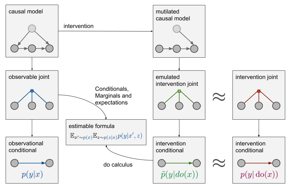
The new panel called "estimable formula" shows the equivalent expression for $\tilde{p}(y\vert do(x))$ obtained as a result of the derivation including several do-calculus rules. Notice how the variable $z$ which is completely irrelevant if you only care about $p(y\vert x)$ is now needed to perform causal inference. If we can't observe $z$ we can still do supervised learning, but we won't be able to answer causal inference queries $p(y\vert do(x))$.
How do I know my causal model is right or wrong?
You can never fully verify the validity and completeness of your causal diagram based on observed data alone. However, there are certain aspects of the causal model which are empirically testable. In particular, the causal diagram implies certain conditional independence or dependence relationships between sets of variables. These dependencies or independencies can be empirically tested, and if they are not present in the data, that is an indication that your causal model is wrong. Taking this idea forward you can attempt to perform full causal discovery: attempting to infer the causal model or at least aspects of it, from empirical data.
But the bottom line is: a full causal model is a form of prior knowledge that you have to add to your analysis in order to get answers to causal questions without actually carrying out interventions. Reasoning with data alone won't be able to give you this. Unlike priors in Bayesian analysis - which are a nice-to-have and can improve data-efficiency - causal diagrams in causal inference are a must-have. With a few exceptions, all you can do without them is running randomized controlled experiments.
Summary
Causal inference is indeed something fundamental. It allows us to answer "what-if-we-did-x" type questions that would normally require controlled experiments and explicit interventions to answer. And I haven't even touched on counterfactuals which are even more powerful.
You can live without this in some cases. Often, you really just want to do normal inference. In other applications such as model-free RL, the ability to explicitly control certain variables may allow you to sidestep answering causal questions explicitly. But there are several situations, and very important applications, where causal inference offers the only method to solve the problem in a principled way.
I wanted to emphasize again that this is not a question of whether you work on deep learning or causal inference. You can, and in many cases you should, do both. Causal inference and do-calculus allows you to understand a problem and establish what needs to be estimated from data based on your assumptions captured in a causal diagram. But once you've done that, you still need powerful tools to actually estimate that thing from data. Here, you can still use deep learning, SGD, variational bounds, etc. It is this cross-section of deep learning applied to causal inference which the recent article with Pearl claimed was under-explored.
UPDATE: In the comments below people actually pointed out some relevant papers (thanks!). If you are aware of any work, please add them there.