Unsupervised Feature Learning in Video: Learning to Linearize

I've just finished reading a paper that will be presented at NIPS this year. I think it's a super interesting topic, the paper is part of a recent trend to focus on exploiting temporal information in video in an unsupervised way. So I decided to write about it here. The more I wrote, the more this post has turned into a criticism of the specifics of the paper - I'm sorry. The paper is:

Ross Goroshin, Michael Mathieu, Yann LeCun (NIPS 2015) Learning to Linearize Under Uncertainty

I think this paper has two main ideas in there, I see them as independent, for reasons explained below:

1. a new penalty function that aims at regularising the second derivative of the trajectory the latent representation traces over time. I see this as a generalisation of the slowness principle or temporal constancy, more about this in the next section.

2. A new autoencoder-like method to predict future frames in video. Video is really hard to forward-predict with non-probabilistic models because high level aspects of video are genuinely uncertain. For example, in a football game, you can't really predict whether the ball will hit the goalpost, but the results might look completely different visually. This, combined with L2 penalties often results in overly conservative, blurry predictions. The paper improves things by introducing extra hidden variables, that allow the model to represent uncertainty in its predictions. More on this later.

Inductive bias: penalising curvature

The key idea of this paper is to learn good distributed representations of natural images from video in an unsupervised way. Intuitively, there is a lot of information contained in video, which is lost if you scramble the video and look at statistics individual frames only. The race is on to develop the right kind of prior and inductive bias that helps us fully exploit this temporal information. This paper presents a way, which is called learning to linearise (I'm going to call this L2L).

Naturally occurring images are thought to reside on some complex, nonlinear manifold whose intrinsic dimension is substantially lower than the number of pixels in an image. It is then natural to think about video as a journey on this manifold surface, along some smooth path. Therefore, if we aim to learn good generic features that correspond to coordinates on this underlying manifold, we should expect that these features vary in a smooth fashion over time as you play the video.

L2L uses this intuition to motivate their choice of an objective function that penalises a scale-invariant measure of curvature over time. In a way it tries to recover features that transform nearly linearly as time progresses and the video is played.

In their notations, $x_{t}$ denotes the data in frame $t$, which is transformed by a deep network to obtain the latent representation $z_{t}$. The penalty for the latent representation is as follows.

$$-\sum_{t} \frac{(z_t - z_{t-1})^{T}(z_{t+1} - z_{t})}{|z_t - z_{t-1}||z_{t+1} - z_{t}|}$$

The expression above has a geometric meaning as the cosine of the angle between the vectors $(z_t - z_{t-1})$ and $(z_{t+1} - z_{t})$. The penalty is minimised if these two vectors are parallel and point in the same direction. In other words the penalty prefers when the latent feature representation keeps its momentum and continues along a linear path - and it does not like sharp turns or jumps. This seems like a sensible prior assumption to build on.

L2L is very similar to another popular inductive bias used in slow feature analysis: the temporal slowness principle. According to this principle, the most relevant underlying features don't change very quickly. The slowness principle has a long history both in machine learning and as a model of human visual perception. In SFA one would minimise the following penalty on the latent representation:

$$\sum_{t} (z_t - z_{t-1})^{2},$$

where the square is applied component-wise. There are additional constraints in SFA, more about this later. We can understand the connection between SFA and this paper's penalty if we plot the penalty for a single hidden feature $z_{t,f}$ at time $t$, keeping all other features and values at neighbouring timesteps constant. This is plotted in the figure below (scaled and translated so the objectives line up nicely).

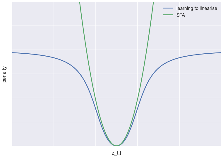
As you can see, both objectives have a minimum at the same location: they both try to force $z_{t,f}$ to linearly interpolate between the neighbouring timesteps. However, while SFA has a quadratic penalty, the learning to linearise objective tapers off at long distances. Compare this to Tukey's loss function used in outlier-resistant robust regression.

Based on this, my prediction is that compared to SFA, this loss function is more tolerant of outliers, which in the temporal domain would mean abrupt jumps in the latent representation. So while SFA is equivalent to assuming that the latent features follow a Brownian-motion-like Ornstein–Uhlenbeck process, I'd imagine this prior corresponds to something like a jump diffusion process (although I don't think the analogy holds mathematically).

Which one of these inductive biases/priors are better at exploiting temporal information in natural video? Slow Brownian motion, or nearly-linear trajectories with potentially a few jumps Unfortunately, don't expect any empirical answer to that from the paper. All experiments seem to be performed on artificially constructed examples, where the temporal information is synthetically engineered. Nor there is any real comparison to SFA.

Representing predictive uncertainty with auxillary variables

While the encoder network learns to construct smoothly varrying features $z_t$, the model also has a decoder network that tries to reconstruct $x_t$ and predict subsequent frames. This, the authors agree, is necessary in order for $z_t$ to contain enough relevant information about the frame $x_t$ (more about whether or not this is necessary later). The precise way this decoding is done has a novel idea as well: minimising over auxillary variables.

Let's say our task is to predict a future frame $x_{t+k}$ based on the latent representation $z_{t}$. The problem is, this is a very hard problem. In video, just like in real life, anything can happen. Imagine you're modelling soccer footage, and the ball is about to hit the goalpost. In order to predict the next frames, not only do we have to know about natural image statistics, we also have to be able to predict whether the goal is in or not. An optimal predictive model would give a highly multimodal probability distribution as its answer. If you use the L2 loss with a deterministic feed-forward predictive network, it's likely to come up with a very blurry image, which would correspont to the average of this nasty multimodal distribution. This calls for something better, either a smarter objective function, or a better way of representing predictive uncertainty.

The solution the authors gave is to introduce hidden variables $\delta_{t}$, that the decoder network also receives as input in addition to $z_t$. For each frame, $\delta_t$ is optimised so that only the best possible reconstruction is taken into account in the loss function. Thus, the decoder network is allowed to use $\delta$ as a source of non-determinism to hedge its bets as to what the contents of the next frame will be. This is one step closer to the ideal setting where the decoder network is allowed to give a full probability distribution of possibilities and then is evaluated using a strictly proper scoring rule.

This inner loop minimisation (of $\delta$) looks very tedious, and introduces a few more parameters that may be hard to set. The algorithm is reminiscent of the E-step in expectation-maximisation, and also very similar to the iterated closest point algorithm Andrew Fitzgibbon talked about in his tutorial at BMVC this year.

In his tutorial, Andrew gave examples where jointly optimising model parameters and auxiliary variables ($\delta$) is advantageous, and I think the same logic applies here. Instead of the inner loop, simultaneous optimisation helps fixing some pathologies, like slow convergence near the optimum. In addition, Andrew advocates exploiting the sparsity structure of the Hessian to implement efficient second-order gradient-based optimisation methods. These tricks are explained in paragraphs around equation 8 in (Prasad et al, 2010).

Predictive model: Is it necessary?

On a more fundamental level, I question whether the predictive decoder network is really a necessary addition to make L2L work.

The authors observe that the objective function is minimised by the "trivial" solutions $z_{t} = at + b$, where $a,b$ can be arbitrary constants. They then say that in order to make sure features do something more than just discover some of these trivial solutions, we also have to include a decoder network, that uses $z_t$ to predict future frames. I believe this is not necessary at all.

Because $z_t$ is a deterministic function of $x_t$, and $t$ is not accessible to $z_{t}$ in any other way than through inferring it from $x_t$, as long as $a\neq 0$, the linear solutions are not trivial at all. If the network discovers $z_{t} = at, a\neq 0$, you should in fact be very happy (assuming a single feature). The only problems with trivial solutions occur when $z_{t} = b$ ($z$ doesn't depend on the data at all) or when $z$ is multidimensional and several redundant features are sensitive to exactly the same thing.

These trivial solutions could be avoided the same way they are avoided in SFA, by constraining the overall spatial covariance of $z_{t}$ over the videoclip to be $I$. This would force each feature to vary at least a little bit with data- hence avoiding the trivial constant solutions. It would also force features to be linearly decorrelated - solving the redundant features problem.

So I wonder if the decoder network is indeed a necessary addition to the model. I would love to encourage the authors to implement their new hypothesis of a prior both with and without the decoder. They may already have tried it without and found it really didn’t work, so it might just be a matter of including those results. This would in turn allow us to see SFA and L2L side-by-side, and learn something about whether and why their prior is better than the slowness principle. Certainly the article provides food for thought.