On Information Theoretic Bounds for SGD
Few days ago we had a talk by Gergely Neu, who presented his recent work:
I'm writing this post mostly to annoy him, by presenting this work using super hand-wavy intuitions and cartoon figures. If this isn't enough, I will even find a way to mention GANs in this context.
But truthfully, I'm just excited because for once, there is a little bit of learning theory that I half-understand, at least at an intuitive level, thanks to its reliance on KL divergences and the mutual information.
A simple guessing game
Let's start this with a simple thought experiment to illustrate why and how mutual information may be useful in describing an algorithm's ability to generalize. Say we're given two datasets, $\mathcal{D}_{train}$ and $\mathcal{D}_{test}$, of the same size for simplicity. We play the following game: we both have access to $\mathcal{D}_{train}$ and $\mathcal{D}_{test}$, and we both know what learning algorithm, $\operatorname{Alg}$ we're going to use.
Now I toss a coin and I keep the result (recorded as random variable $Y$) a secret. If it's heads, I run $\operatorname{Alg}$ on the training set $\mathcal{D}_{train}$. If it's tails, I run $\operatorname{Alg}$ on the test data $\mathcal{D}_{test}$ instead. I don't tell you which of these I did, I only reveal to you the final parameter value $W$. Can you guess, just by looking at $W$, whether I trained on training or test data?
If you cannot guess $Y$, that means that the algorithm returns the same random $W$ irrespective of whether you train it on training or test data. So the training and test losses become interchangeable. This implies that the algorithm will generalize very well (on average) and not overfit to the data it's trained on.
The mutual information, in this case between $W$ and $Y$ quantifies your theoretical ability to guess $Y$ from $W$. The higher this value is, the easier it is to tell which dataset the algorithm was trained on. If it's easy to reverse engineer my coin toss from parameters, it means that the algorithm's output is very sensitive to the input dataset it's trained on. And that likely implies poor generalization.
Note by: an algorithm generalizing well on average doesn't mean it works well on average. It just means that there won't be a large gap between the expected training and expected test error. Take for example an algorithm returns a randomly initialized neural network, without even touching the data. That algorithm generalizes extremely well on average: it does just as poorly on test data as it does on training data.
Illustrating this in more detail
Below is an illustration of my thought experiment for SGD.
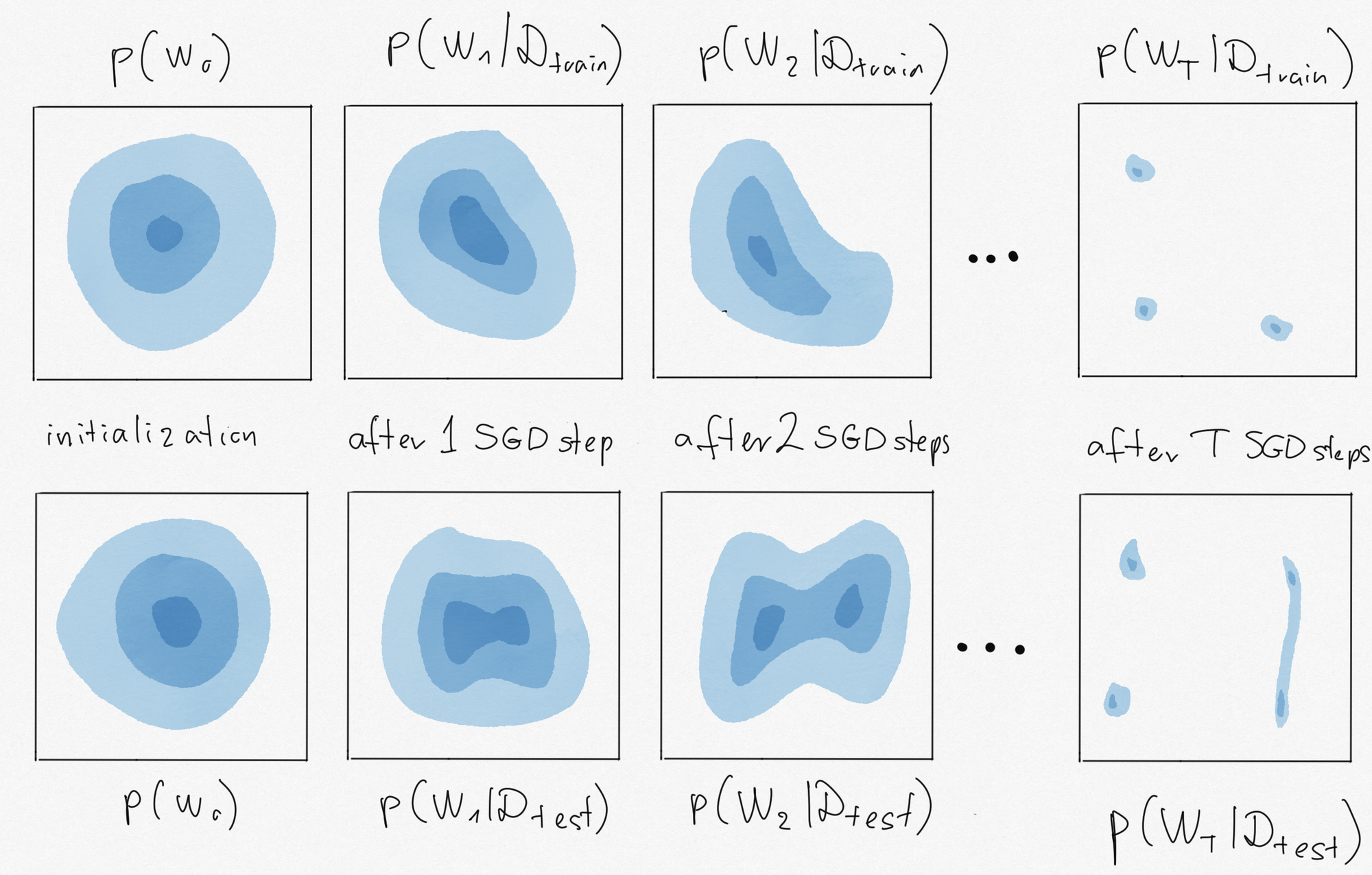
In the top row, I doodled the distribution of the parameter $W_t$ at various timesteps $t=0,1,2,\ldots,T$ of SGD. We start the algorithm by initializing $W$ randomly from a Gaussian (left panel). Then, each stochastic gradient update changes the distribution of $W_t$ a bit compared to the distribution of $W_{t-1}$. How the shape of the distribution changes depends on the data we use in the SGD steps. In the top row, let's say I ran SGD on $\mathcal{D}_{train}$ and in the bottom, I run it on $\mathcal{D}_{test}$. The distibutions $p(W_t\vert \mathcal{D})$ I drew here describe where the SGD iterate is likely to be after $t$ steps of SGD started from random initialization. They are not to be confused with Bayesian posteriors, for example.
We know that running the algorithm on the test set would produce low test error. Therefore, sampling a weight vector $W$ from $p(W_T\vert \mathcal{D}_{test})$ would be great if we could do that. But in practice, we can't train on the test data, all we have the ability to sample from is $p(W_T\vert \mathcal{D}_{train})$. So what we'd like for good generalization, is if $p(W_T\vert \mathcal{D}_{test})$ and $p(W_T\vert \mathcal{D}_{train})$ were as close as possible. The mutual information between $W_T$ and my coinflip $Y$ measures this closeness in terms of the Jensen-Shannon divergence:
$$
\mathbb{I}[Y, W_T] = \operatorname{JSD}[p(W_T\vert \mathcal{D}_{test})\|p(W_T\vert \mathcal{D}_{train})]
$$
So, in summary, if we can guarantee that the final parameter an algorithm comes up with doesn't reveal too much information about what dataset it was trained on, we can hope that the algorithm has good generalization properties.
Mutual Inforrmation-based Generalization Bounds
These vague intuitions can be formalized into real information-theoretic generalization bounds. These were first presented in a general context in (Russo and Zou, 2016) and in a more clearly machine learning context in (Xu and Raginsky, 2017). I'll give a quick - and possibly somewhat handwavy - overview of the main results.
Let $\mathcal{D}$ and $\mathcal{D}'$ be random datasets of size $n$, drawn i.i.d. from some underlying data distribution $P$. Let $W$ be a parameter vector, which we obtain by running a learning algorithm $\operatorname{Alg}$ on the training data $\mathcal{D}$: $W = \operatorname{Alg}(\mathcal{D})$. The algorithm may be non-deterministic, i.e. it may output a random $W$ given a dataset. Let $\mathcal{L}(W, \mathcal{D})$ denote the loss of model $W$ on dataset $\mathcal{D}$. The expected generalization error of $\operatorname{Alg}$ is defined as follows:
$$
\text{gen}( \operatorname{Alg}, P) = \mathbb{E}_{\mathcal{D}\sim P^n,\mathcal{D}'\sim P^n, W\vert \mathcal{D}\sim \operatorname{Alg}(\mathcal{D})}[\mathcal{L}(W, \mathcal{D}') - \mathcal{L}(W, \mathcal{D})]
$$
If we unpack this, we have two datasets $\mathcal{D}$ and $\mathcal{D}'$, the former taking the role of the training dataset, the latter of the test data. We look at the expected difference between the training and test losses ($\mathcal{L}(W, \mathcal{D})$ and $\mathcal{L}(W, \mathcal{D}')$), where $W$ is obtained by running $\operatorname{Alg}$ on the training data $\mathcal{D}$. The expectation is taken over all possible random training sets, test sets, and over all possible random outcomes of the learning algorithm.
The information theoretic bound states that for any learning algorithm, and any loss function that's bounded by $1$, the following inequality holds:
$$
gen(\operatorname{Alg}, P) \leq \sqrt{\frac{\mathbb{I}[W, \mathcal{D}]}{n}}
$$
The main term in the RHS of this bound is the mutual infomation between the training data \mathcal{D} and the pararmeter vector $W$ the algorithm finds. It essentially quantifies the number of bits of information the algorithm leaks about the training data into the parameters it learns. The lower this number, the better the algorithm generalizes.
Why we can't apply this to SGD?
The problem with applying these nice, intuitive bounds to SGD is that SGD, in fact, leaks too much information about the specific minibatches it is trained on. Let's go back to my illustrative example of having to guess if we ran the algorithm on training or test data. Consider the scenario where we start form some parameter value $w_t$ and we update either with a random minibatch of training data (blue) or a random minibatch of test data (orange).
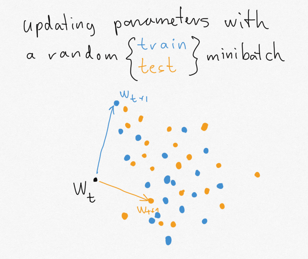
Since the training and test datasets are assumed to be of finite size, there are only a finite number of possible minibatches. Each of these minibatches can take the parameter to a unique new location. The problem is, the set of locations you can reach with one dataset (blue dots) does not overlap with the set of locations you can reach if you update with the other dataset (orange dots). Suddenly, if I give you $w_{t+1}$, you can immediately tell if it's an orange or blue dot, so you can immediately reconstruct my coinflip $Y$.
In the more general case, the problem with SGD in the context of information-theoretic bounds is that the amount of information SGD leaks about the dataset it was trained on is high, and in some cases may even be infinite. This is actually related to the problem that several of us noticed in the context of GANs, where the true and fake distributions may have non-overlapping support, making the KL divergence infinite, and saturating out the Jensen-Shannon divergence. The first trick we came up with to solve this problem was to smooth things out by adding Gaussian noise. Indeed, adding noise is key what researches have been doing to apply these information-theoretic bounds to SGD.
Adding noise to SGD
The first thing people did (Pensia et al, 2018) is to study a noisy cousin of SGD: stochastic gradient Langevin dynamics (SGLD). SGDL is like SGD but in each iteration we add a bit of Gaussian noise to the parameters in addition to the gradient update. To understand why SGLD leaks less information, consider the previous example with the orange and blue point clouds. SGLD makes those point clouds overlap by convolving them with Gaussian noise.
However, SGLD is not exactly SGD, and it's not really used as much in practice. In order to say something about SGD specifically, Neu (2021) did something else, while still relying on the idea of adding noise. Instead of baking the noise in as part of the algorithm, Neu only adds noise as part of the analysis. The algorithm being analysed is still SGD, but when we measure the mutual information we will measure the mutual information between $\mathbb{I}[W + \xi; \mathcal{D}]$, where $\xi$ is Gaussian noise.
I leave it to you to check out the details of the paper. While the findings fall short of explaining whether SGD have any tendency to find solutions that generalise well, some of the results are nice and interpretable: they connect the generalization of SGD to the noisiness of gradients as well as the smoothness of the loss along the specific optimization path that was taken.