Instance Noise: A trick for stabilising GAN training

Generative Adversarial Networks (GANs) are notoriously hard to train. In a recent paper, we presented an idea that might help remedy this.

Our intern Casper spent the summer working with GANs, resulting in a paper which appeared on arXiv this week. One particular technique did us great service: instance noise. It's not the main focus of Casper's paper, so the details have been relegated to an Appendix. We thought it's a good idea to summarise it here, giving a few more details. Naturally, I think the full paper is also worth a read, there are a few more interesting things in there:

• Casper Kaae Sønderby, Jose Caballero, Lucas Theis, Wenzhe Shi and Ferenc Huszár (2016) Amortised MAP Inference for Image Super-Resolution

Instance noise

Summary

• we think a major reason for GANs' instability may be that the generative distributions are weird, degenerate, and their support don't generally overlap with the true data distribution.
• this makes the nice theory break down and may lead to unstable behaviour
• we suggest adding noise to both real and synthetic data during training might help overcome these problems
• in this note we motivate this technique and illustrate in a few figures how it helps training

GANs should work.

There are different ways to think about GANs: you can approach it from a game theoretic view of seeking Nash equilibrium (Salimans et al, 2016), or you can treat it as an E-M like iterative algorithm where the discriminator's job is likelihood ratio estimation (Mohamed et al, 2016, Uehara et al, 2016, Nowozin et al). If you've read my earlier posts, it should come as no surprise that I subscribe to the latter view.

Consider the following idealised GAN algorithm, each iteration consisting of the following steps:

• we train the discriminator $D$ via logistic regression between our generative model $q_\theta$ vs true data $p$, until convergence
• we extract from $D$ an estimate of the logarithmic likelihood ratio $s(y) = \log \frac{q_\theta(y)}{p(y)}$
• we update $\theta$ by taking a stochastic gradient step with objective function $\mathbb{E}_{y\sim q_\theta}s(y)$

If $q_\theta$ and $p$ are well-conditioned distributions in a low-dimensional space, this algorithm performs gradient descent on an approximation to the KL divergence, so it should converge.

So why don't they?

Crucially, the convergence of this algorithm relies on a few assumptions never really made explicit that don't always hold:

1. that the log-likelihood-ratio $\log \frac{q_\theta(y)}{p(y)}$ is finite, or
2. that the Jensen-Shannon divergence $\operatorname{JS}[q_\theta|p]$ is a well-behaved function of $\theta$ and
3. that the Bayes-optimal solution to the logistic regression problem is unique: there is a single optimal discriminator that does a much better job than any other classifier.

In the paper we argued that in real-world situations neither of these holds, mainly because $q_\theta$ and $p$ are concentrated distributions whose support may not overlap. In image modelling, distribution of natural images $p$ is often assumed to be concentrated on or around a lower-dimensional manifold. Similarly, $q_\theta$ is often degenerate by construction. The odds that the two distributions share support in high-dimensional space, especially early in training, are very small.

If $q_\theta$ and $p$ have non-overlapping support, then

1. the log-likelihood-ratio and therefore KL divergence is infinite and not well defined
2. the Jensen-Shannon divergence is saturated so its maximum value: To see why, consider the mutual information interpretation of JS divergence. If the two distributions $q_\theta$ and $p$ have no overlap, they can be separated perfectly, so mutual information is maximal. If this is the case, $JS$ is locally constant in $\theta$.
3. the discriminator is extremely prone to overfitting: there may be a large set of near-optimal discriminators whose loss is very close to the Bayes optimum. Thus, for a fixed $q_\theta$ and $p$, training the discriminator $D$ might lead to a different near-optimal solution each time depending on initialisation. And, each of these near-optimal solutions might provide very different gradients (or no useful gradients at all) to the generator.

How to fix this?

The main ways to avoid these pathologies involve making the discriminator's job harder. Why? The $JS$ divergence is constant locally in $\theta$, but it doesn't mean that the variational lower bound also has to be constant. Indeed, if you cripple the discriminator so the lower bound is not tight, you may end up with a non-constant function of $\theta$ that will roughly guide you to the right direction.

An example of this crippling is that in most GAN implementations the discriminator is only partially updated in each iteration, rather than trained until convergence. This extreme form of early stopping is a form of regularisation that prevents the discriminator from overfitting.

Another way to cripple the discriminator is adding label noise, or equivalently, one-sided label smoothing as introduced by Salimans et al, (2016). In this technique the labels in the discriminator's training data are randomly flipped. Let's illustrate this technique in two figures.

The classifiaction view:

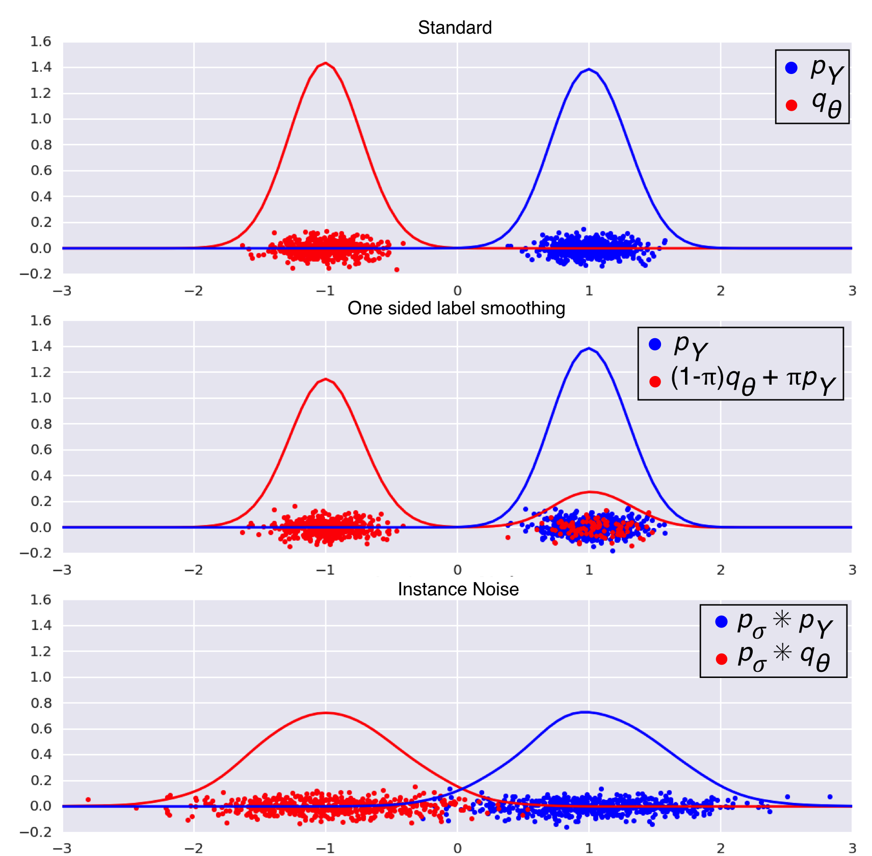
The top panel shows two almost perfectly separable distributions $q_\theta$ and $p$ (it is called $p_Y$ in the paper). Notice how the large gap between the distributions means that there are large number of possible classifiers that tell the two distributions apart and achieve similar logistic loss. The Bayes-optimal classifier may not be unique, and the set of near-optimal classifiers is very large and diverse.

In the middle panel we show the effect of \emph{one sided label smoothing} or equivalently, adding label noise. In this technique, the labels of some real data samples $x\sim p$ are flipped so the discriminator is trained thinking they were samples from $q_\theta$. The discriminator indeed has a harder task now. However, the likelhiood ratio $\log \frac{p}{(1-\pi) q\theta + \pi p}$ is still not well-defined. Also, although discriminators have a harder job, they are all punished evenly: there is no way for the discriminator to be smart about handling label noise. Adding label noise doesn't change the structure of the logistic regression loss landscape dramatically, it mainly just pushes everything up. Hence, there are still a large number of near-optimal discriminators. Adding label noise still does not allow us to pinpoint a single unique Bayes-optimal classifier. The JS divergence is not saturated to its maximum level anymore, but it is still locally constant in $\theta$.

The last panel shows the technique we propose, whereby we add noise to samples from both $q_\theta$ and $p$. We use convolution $p_\sigma \ast q_\theta$ to denote additive noise. As a result, the noisy distributions now overlap, the log-likelihood-ratio $\log \frac{p_\sigma \ast p}{p_\sigma \ast q_\theta}$ is well-behaved, and the JS divergence between the two noisy distributions is a non-constant function of $\theta$.

The graphical model view:

An alrernative way to think about instance noise vs. label noise is via graphical models. The following three graphical models define joint distributions, parametrised by $\theta$. The GAN algorithm tries to adjust $\theta$ so as to minimise the mutual information between the highlighted nodes in these graphical models:

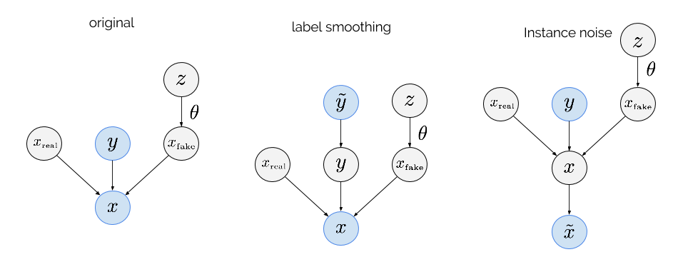
Here's what the variables are:

• $z$ is the latent variable we feed into the generator (in our image superresolution, this was the low-resolution image)
• $x_{fake}$ is a synthetic sample we draw from the generator $q_\theta$, by squashing $z$ through a nonlinearity parametrised by $\theta$
• $x_{real}$ is a real data sample, drawn from $p$
• $y$ is a binary label, a coinflip, sampled from a Bernoulli distribution with parameter $0.5$
• $x$ is a datapoint that the discriminator would see: depending on $y$, it's either a copy of $x_{real}$ or $x_{fake}$
• $\tilde{y}$ is a noisy label that is the same as $y$ most of the time, but they can be randomly flipped.
• $\tilde{x}$ is a noisy version of $x$, generated by adding noise $\nu \sim p_\sigma$ to x.

In this joint distribution, vanilla GANs minimise is the mutual information $\mathbb{I}[x,y]$ which corresponds to JS divergence. If the distributions of $x_{fake}$ and $x_{real}$ have no overlap, $y$ is a deterministic function of $x$ and therefore the mutual information is maximal. Hence, in this scenario, the objective function is theoretically constant in $\theta$.

The second panel shows the effect of label smoothing, or, adding label noise. Now the discriminator is trained on randomly flipped labels $\tilde{y}$ instead of the real labels $y$. The GAN algorithm can be thought of as trying to minimise $\mathbb{I}[x,\tilde{y}]$. It is not hard to see that, in situations where $y$ is a deterministic function of $x$, then this mutual information is also constant with respect to $\theta$.

In the instance noise trick, the discriminator sees the correct labels $y$, but its input is the noisy $\tilde{x}$. We think that $\mathbb{I}[\tilde{x},y]$ is a much better objective function to target. Even when $\mathbb{I}[y;x]$ is saturated, $\mathbb{I}[\tilde{x},y]$ still depends on $\theta$ in a non-trivial and meaningful way. If the noise distribution $p_\sigma$ is something like a Gaussian, adding noise can be thought of as a way to measure how far away $q$ and $p$ are from each when they don't overlap.

The divergence view

Finally, there's a way to understand label noise from the perspective of minimising divergences. Using a GAN algorithm we can construct algorithms that minimise the following family of divergences:

$$
d_\sigma(q_\theta|p) = KL[p_\sigma \ast q_\theta|p_\sigma \ast p],
$$

or

$$
d_{\sigma,JS}(q_\theta|p) = JS[p_\sigma \ast q_\theta|p_\sigma \ast p],
$$

where $\sigma$ is the parameter of the noise distribution. Importantly, these divergences are still convex and have a global minimum when $q_\theta = p$. Obviously, as the noise level $\sigma$ increases, the fine details of the distribution are "blurred out" so the divergences are expected to become less sensitive to fine patterns.

Does it work?

We tried this technique in the context of GANs for image superresolution, and we found it stabilises training, as predicted. We used additive Gaussian white noise whose variance parameter $\sigma$ we annealed linearly during training. The figure below shows that the discriminator's performance is kept in check by the added noise throughout training:

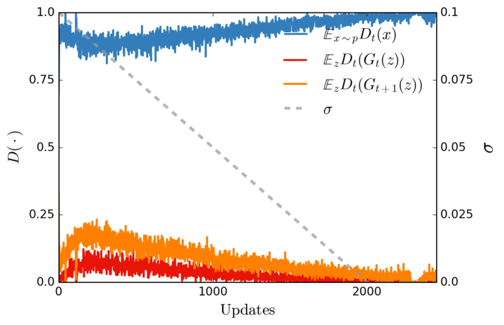
The blue curve shows the average probability the discriminator assigns to real data, the red the probability it assigns to synthetic data. If the discriminator was winning, these probabilities would always be $0.0$ and $1.0$, but the noise makes the discriminator's job harder. The orange curve shows the probability the current discriminator $D_t$ assigns to new fake data, after the generator is updated ($G_{t+1}$). As expected, the orange curve is always above the red one, which means that the current approximation of $d_\sigma(q_\theta|p)$ had been improved.

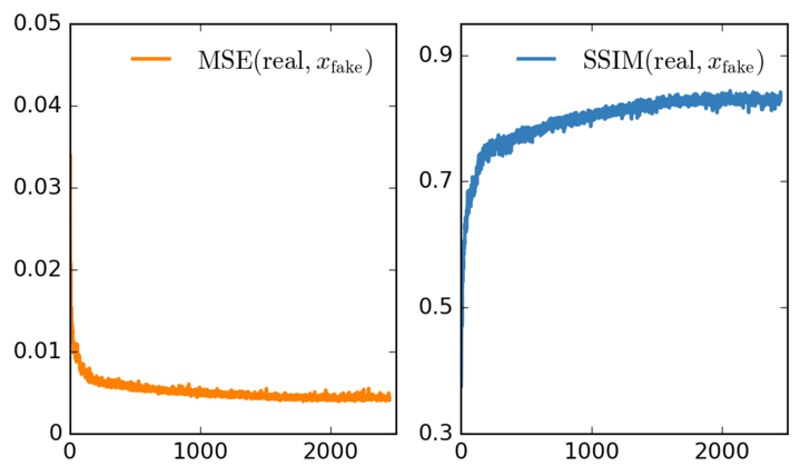
Another way to show that convergence is happening is to look at the average SSIM and MSE values during training. This is only possible because we trained the network for superresolution, so we actually always had a ground truth image to compare to. Both metrics improve steadily as the figures show:

Conclusion

Instance noise is a theoretically motivated way to remedy the poor convergence properties of GANs. We have not tested it extensively in the context of generative modeling, but we think it should help there also. Let us know if you have any experience with similar techniques.