GANs are Broken in More than One Way: The Numerics of GANs
Last year, when I was on a mission to "fix GANs" I had a tendency to focus only on what the loss function is, and completely disregard the issue of how do we actually find a minimum. Here is the paper that has finally challenged that attitude:
- Mescheder, Nowozin, Geiger (2017): The Numerics of GANs
I reference Marr's three layers of analysis a lot, and I enjoy thinking about problems at the computational level: what is the ultimate goal we do this for? I was convinced GANs were broken at this level: they were trying to optimize for the wrong thing or seek equilibria that don't exist, etc. This is why I enjoyed f-GANs, Wasserstein GANs, instance noise, etc, while being mostly dismissive of attempts to fix things at the optimization level, like DCGAN or improved techniques (Salimans et al. 2016). To my defense, in most of deep learning, the algorithmic level is sorted: stochastic gradient descent. You can improve on it, but it's not broken, it doesn't usually need fixing.
But after reading this paper I had a revelation:
GANs are broken at both the computational and algorithmic levels.
Even if we fix the objectives, we don't have algorithmic tools to actually find solutions.😱
Summary of this post
- as it is now expected of my posts, I am going to present the paper through a slightly different lens
- I introduce the concept of conservative vs non-conservative vector fields, and highlight some of their properties
- I then explain how consensus optimization proposed by Mescheder et al can be viewed in this context: it interpolates between a nasty non-conservative field and its well-behaved conservative relaxation
- Finally, as it is also expected of my posts, I also highlight an important little detail, which was not discussed in the paper: how should we do all this in the minibatch setting?
Intro: from GANs to vector fields
GANs can be thought of as a two-player non-cooperative game. One player controls $\theta$ and wants to maximize its payoff $f(\theta, \phi)$, the other controls $\phi$ and seeks to maximize $g(\theta,\phi)$. The game is at a Nash equilibrium when neither player can improve its payoff by changing their parameters slightly. Now we have to design an algorithm to find such a Nash equilibrium.
It seems that there are two separate issues with GANs:
- computational: no Nash equilibrium exists or it may be degenerate (Arjovsky and Bottou 2017, Sønderby et al 2017, blog post).
- algorithmic: we don't have reliable tools for finding Nash equilibria (even though we're now pretty good at finding local optima)
Mescheder et al (2017) address the second issue, and do it very elegantly. To find Nash equilibria, our best tool is simultaneous gradient ascent, an iterative algorithm defined by the following recursion:
$$
x_{t+1} \leftarrow x_t + h v(x_t),
$$
where $x_t = (\theta_t, \phi_t)$ is the state of the game, $h$ is a scalar stepsize and $v(x)$ a the following vector field:
$$
v(x) = \left(\begin{matrix}\frac{\partial}{\partial\theta}f(\theta, \phi)\\\frac{\partial}{\partial\phi}g(\theta, \phi)\end{matrix}\right).
$$
Here is an important observation that may look paradoxical at first: it is natural to think of GAN training as a special case of neural network training, but in fact, it is the other way around:
simultaneous gradient descent is a generalization, rather than a special case, of gradient descent
Non-conservative vector fields
One key difference between ordinary gradient descent and simultaneous gradient descent is that while the former finds fixed points of a conservative vector field, the latter has to deal with non-conservative fields. Therefore, I want to spend most of this blog post talking about this difference and what these terms mean.
A vector field on $\mathbb{R}^n$ is simply a function, $v:\mathbb{R}^n \rightarrow \mathbb{R}^n$, which takes a vector $x$ and outputs another vector $v(x)$ of the same dimensionality.
A vector field we often work with is the gradient of a scalar function, say $v(x) = \frac{\partial}{\partial x} \phi(x)$, where $\phi:\mathbb{R}^n \rightarrow \mathbb{R}$ can be a training objective, energy or loss function. These types of vector fields are very special. They are called conservative vector fields, which essentially translates to "nothing particularly crazy happens". Conservative fields and gradients of scalar functions are a one-to-one mapping: if and only if a vector field $v$ is conservative, is there a scalar potential $\phi$ whose gradient equals $v$.
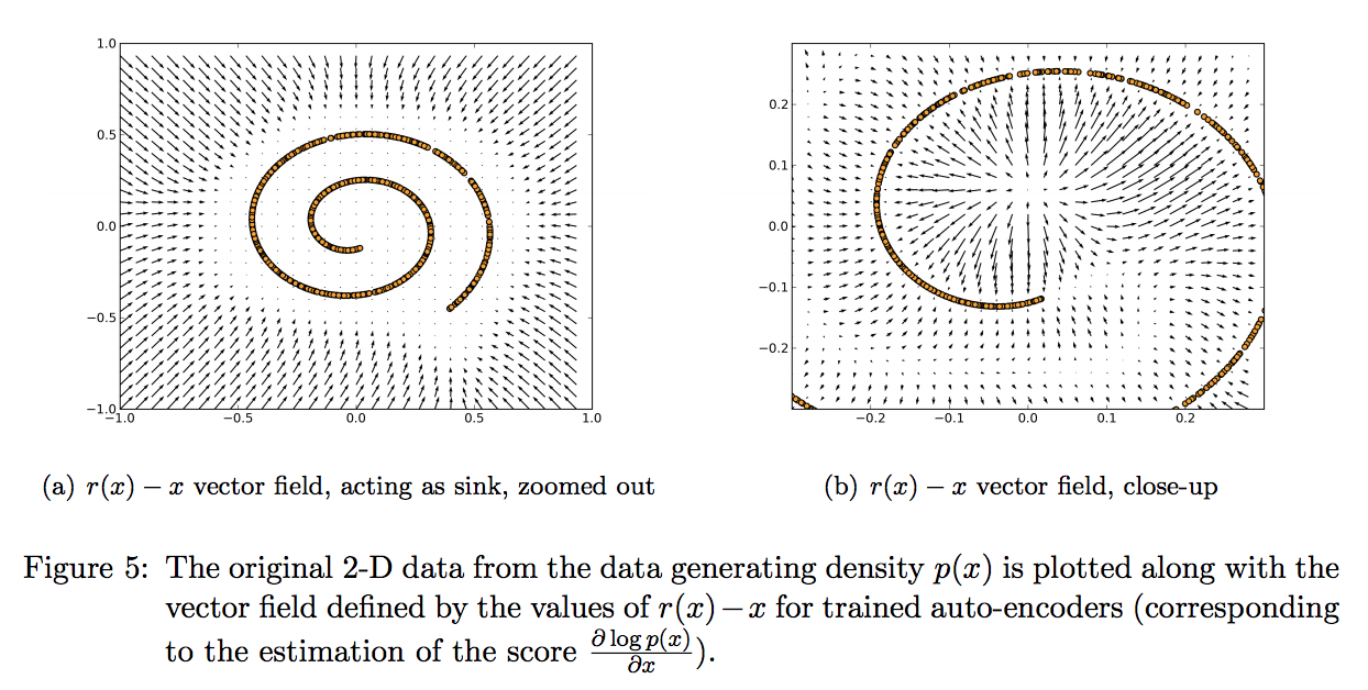
Another vector field we often encounter in machine learning (but don't often think of it as a vector field) is the one defined by an autoencoder. An AE, too, takes as input some vector $x$ and returns another vector $v(x)$ which is the same size. Figure 5 of (Alain and Bengio, 2014) illustrates the vector field of denoising autoencoders trained on 2D data pretty nicely:
A vector field defined by an AE is not necessarily conservative, which basically means that weird things can happen. What kind of weird things? Let's have a look at an extreme example: the constant curl vector field $v(\theta,\phi) = (-\phi, \theta)$, a very typical example of a non-conservative vector field:
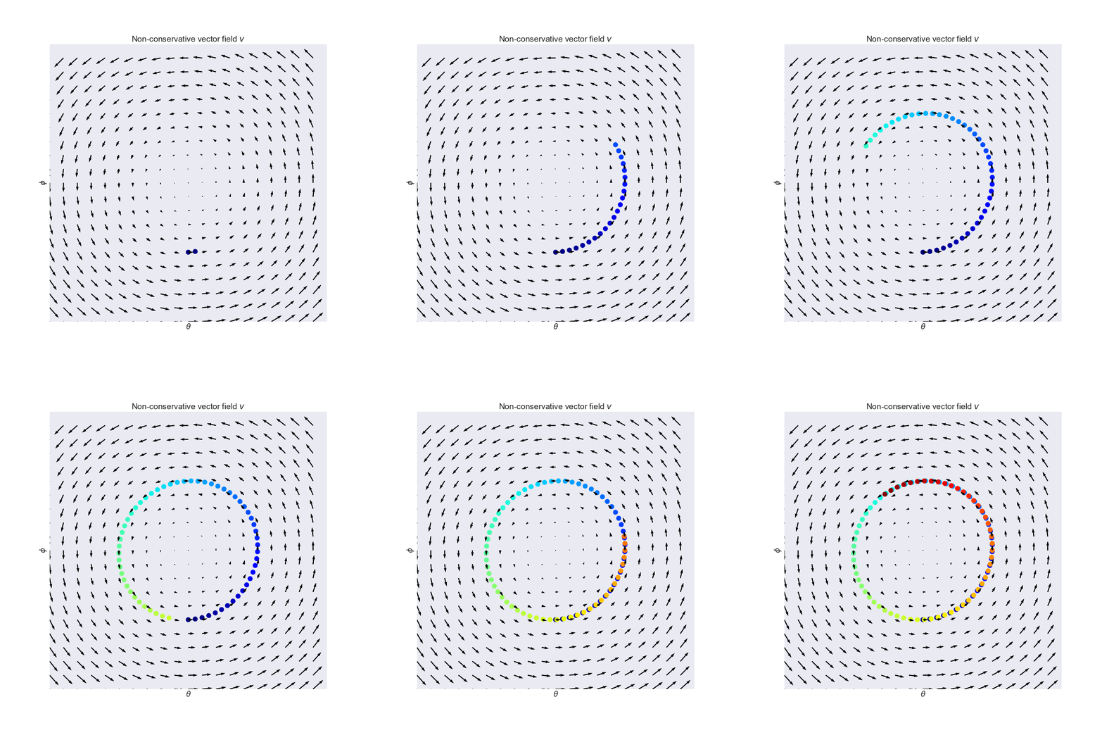
This vector field arises naturally in the zero-sum game where $f(\theta, \phi)=-g(\theta, \phi)=-\theta\phi$. Salimans et al. (2016, Section 3) mention the exact same toy example in the context of GANs. Notice how the vectors point around in circles, and the rotation in the field is visually apparent. Indeed, if you follow the arrows on this vector field (which is what simultaneous gradient descent does), you just end up going in circles, as shown.
Compare this vector field to Escher's impossible tower below. the servants think they are ascending, or descending, but in reality all they do is go around in circles. It is of course impossible to build Escher's tower as a real 3D object. Analogously, it is impossible to express the curl vector field as the gradient of a scalar function.
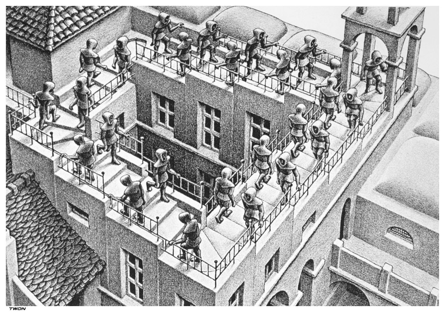
Even though the curl field has an equilibrium at $(\theta, \phi)=(0, 0)$, simultaneous gradient descent will never find it, which is bad news. While we got used to gradient descent always converging to a local minimum, simultaneous gradient descent does not generally converge to equilibria. It can just get stuck in a cycle, and momentum-based variants can even accumulate unbounded momentum and go completely berserk.
Consensus optimization: taming a non-con vector field
The solution proposed by Mescheder et al is to construct a conservative vector field from the original as follows: $-\nabla L(x) := -\frac{\partial}{\partial x}| v(x) |_2^2$. This is clearly conservative since we defined it as the gradient of a scalar function $L$. It is easy to see that this new vector field $-\nabla L$ has the same fix points as $v$. Below I plotted the conservative vector field $-\nabla L$ that corresponds to the curl field above:
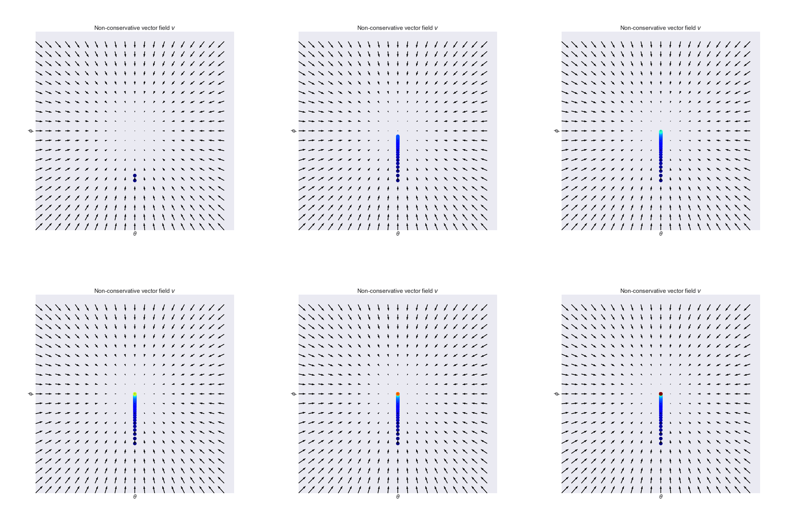
This is great. Familiar gradient descent on $L$ converges to a local minimum, which is a fix point of $v$. The problem now is, we have no control over what kind of fix point we converge to. We seek positive equilibria, but $-\delta L$ can't differentiate between saddle points or equilibria, or between negative or positive equilibria. This is illustrated on this slightly more bonkers vector field $v(\theta, \phi) = (cos(\phi), sin(\theta))$:

On the left-hand plot I annotated equilibria and saddle points. The middle plot shows the conservative relaxation $-\nabla L$ where both saddle points and equilibria are turned to local minima.
So what can we do? We can simply take a linear combination of the original $v$ and it's conservative cousin $-\nabla L$. This is what the combined (still non-conservative) vector field looks like for the curl field (see also the third panel of the figure above):
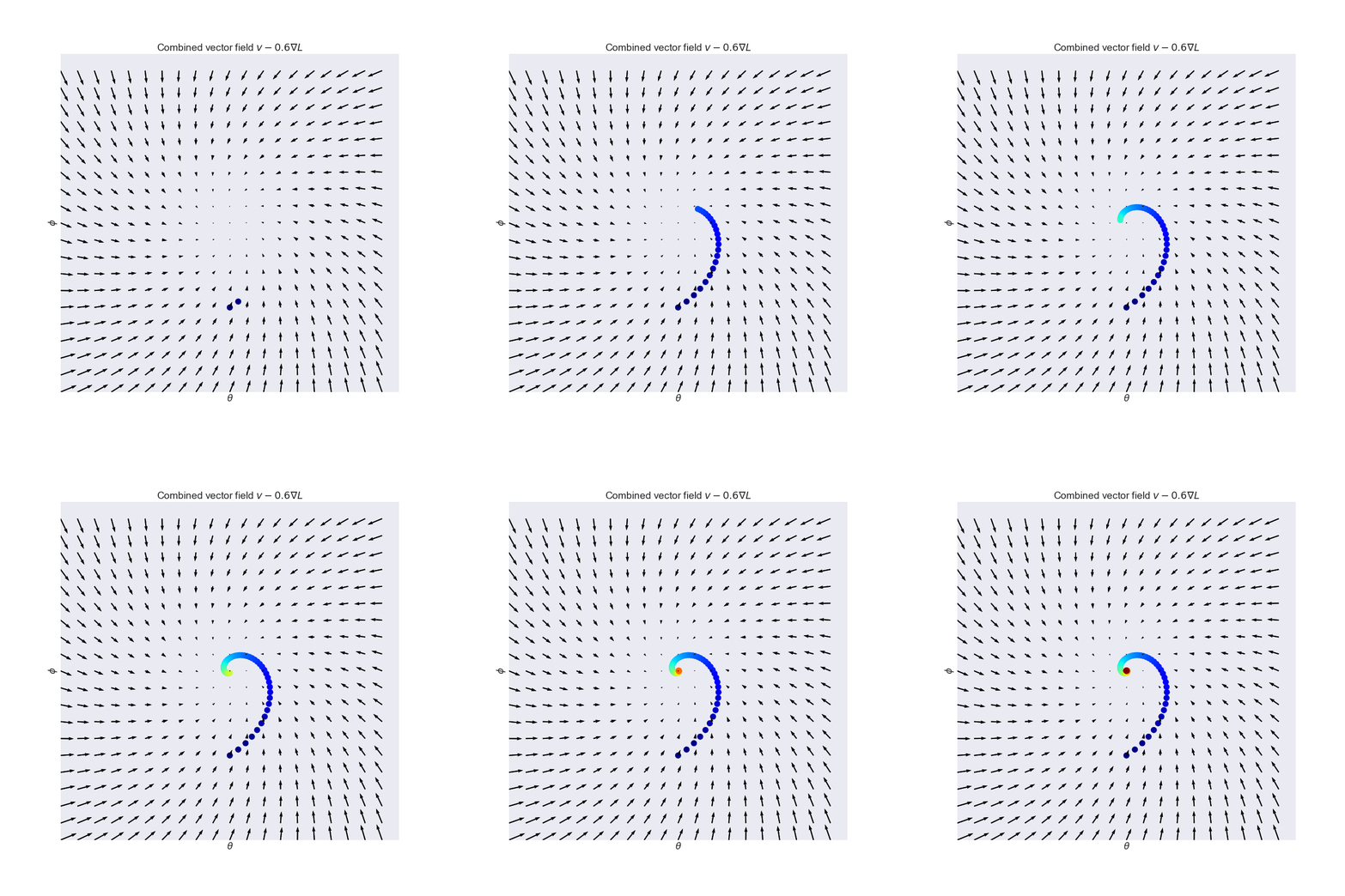
By combining the two fields, we may end up with a slightly better-behaved, but still non-conservative vector field. One way to quantify how well a vector field behaves is to look at eigenvalues of its Jacobian $v'(x)$. The Jacobian is the derivative of the vector field, and for conservative fields it is called the Hessian, or second derivative. Unlike the Hessian, which is always symmetric, the Jacobian of non-conservative fields is non-symmetric, and it can have complex eigenvalues. For example, the Jacobian of the curl field is
$$
v'(x) = \left[\begin{matrix}0&-1\\1&0\end{matrix}\right],
$$
whose eigenvalues are entirely imaginary $+i$ and $-i$.
Mesceder et al show that by combining $v$ with $-\nabla L$, the eigenvalues of the combined field can be controlled (see paper for details), and if we choose a large enough $\gamma$, simultaneous gradient descent will converge to an equilibrium. Hooray!
Sadly, as we increase $\gamma$, we also introduce the spurious equilibria as before. These are equilibria of $v - \gamma\nabla L$ which are in fact only saddle points of $v$. So we can't just crank $\gamma$ up all the way, we have to find a reasonable middle-ground. This is a limitation of the approach, and it is unclear how much of a practical limitation it is.
One more thing: stochastic/minibatch variant
I wanted to mention one more thing which is not discussed in the paper, but I think is important for anyone who would like to play with consensus optimization: how do we implement this with stochastic optimisation and minibatches? Although the paper deals with general games, in the case of a GAN, both $f$ and $g$ are in fact the average of some payoff over datapoints, e.g. $f(\theta, \psi) = \mathbb{E}_x f(\theta, \psi, x)$. Thus, for $L$ we have:
\begin{align}
L(x) &= \left| \frac{\partial f(\theta, \phi)}{\partial \theta} \right|_2^2 + \left| \frac{\partial g(\theta, \phi)}{\partial \theta} \right|_2^2 \\
&= \left| \mathbb{E}_{x}\frac{\partial f(\theta, \phi, x)}{\partial \theta} \right|_2^2 + \left| \mathbb{E}_{x}\frac{\partial g(\theta, \phi, x)}{\partial \theta} \right|_2^2
\end{align}
The problem with this is that it is not immediately trivial how to construct an unbiased estimator for this from a minibatch of samples. Simply taking the norm of the gradient for each datapoint and then averaging will give us a biased estimate, an upper bound by Jensen's inequality. Averaging gradients in the minibatch, and then calculating the norm is still biased, but it is a slightly tighter upper bound.
To construct an unbiased estimator, one can use the following identity:
$$
\mathbb{E}[X]^2 = \mathbb{E}[X^2] - \mathbb{V}[X],
$$
where both the average norm and the population variance can be estimated in an unbiased fashion. I have discussed this with the authors, and I will ask them to leave a comment as to how exactly they did this in the experiment. They also promised to include more details about this in the camera ready version of the paper.
Summary
I really liked this paper, it was a real eye opener. I always thought of the gradient descent-like algorithm we use in GANs as a special case of gradient descent, whereas in fact it is a generalisation. Therefore, the nice properties of gradient descent can't be taken for granted. The paper proposes a general, and very elegant solution. Good job. Let's hope this will fix GANs once and for all.
