Exemplar CNNs and Information Maximization
A few weeks ago I wrote about the then-new paper "Unsupervised Learning by Predicting Noise". In that note, I showed that the method can also be understood from an information maximisation perspective: we seek nonlinear representations of data that have limited entropy (compact) while retain maximal information about the inputs.
In that note, I briefly mentioned another method, exemplar-CNNs, which can also be interpreted this way. As I haven't seen this connection made anywhere, I thought this warrants its own post. Here's the paper:
- Dosovitskiy, Fischer, Springenberg, Riedmiller & Brox (2014) Discriminative Unsupervised Feature Learning with Exemplar Convolutional Neural Networks
Summary of this post
- I provide a very high level overview of the exemplar-CNN training method (as per usual, read the paper for the real thing)
- Then I talk briefly about Variational Information Maximisation, and show that applies to the exemplar-CNN case
- interestingly, exemplar-CNN exploits the fact that we only use a relatively modest subset of training patches, so it makes more sense to represent the distribution of data as an empirical distribution (discrete distribution over finite number of possiblities)
- assuming discreteness, one can derive the exemplar CNN objective as a lower-bound to the mutual information between the seed patch and the representation.
Overview of exemplar CNNs
The technique used by Dosovistkiy et al (2014) is pretty simple: you take a modest number of interesting image patches from an unlabelled dataset, call these seed patches or exemplars. For each patch, you use data-augmentation-like transformations to generate a surrogate class of transformed image patches: you do things like rotations, translations, colour manipulation, etc. For example, this is what this augmented surrogate class looks like for the seed image of a deer (shown in the top-left corner):
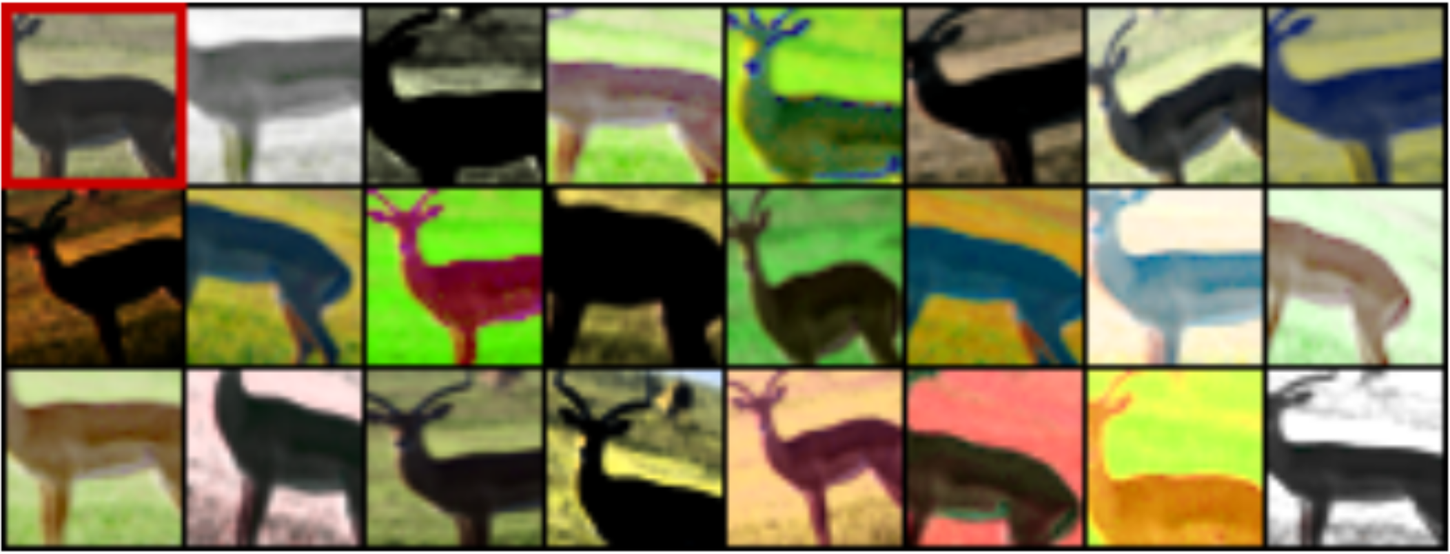
You create this surrogate class for all of your exemplar patches so you end up with as many classes as there were seed patches. Now you train a ConvNet to take a transformed patch and predict the index of the seed image it was generated from. Thus, if you have 8000 seed images, you end up solving a 8000-way classification problem (ergo, you have an 8000-dimensional softmax at the end of your network).
Of course, as the number of seed images increases, training becomes more and more difficult, due to the high-dimensional soft-max in the end. But in reality, the authors show you can get reasonable results using only around 8000 seed patches - at which size the softmax is still managable.
Variational Information Maximisation View
Information Maximisation can be applied in a number of ways to learn representation, depending on what variables you measure information between. To understand exemplar-CNN in this framework, let's consider the following Markov chain:
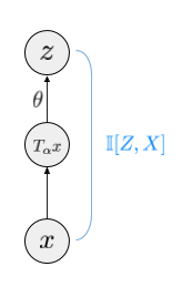
Here, $x$ is the image patch. $T_\alpha x$ is a transformed patch (with the transformation parameter $\alpha$ being randomly sampled). $z = g(T_\alpha x; \theta)$ is a mapping that takes the random image and computes the representation. Thus, the arrow that goes from $T_\alpha x$ to $z$ is in fact a deterministic mapping.
If we think of $z$ as the representation of $x$, it might make sense to maximise the mutual information $\mathbb{I}[X,Z]$. This mutual information can be lower-bounded using the standard variational lower bound on the mutual information (see e.g. Barber and Agakov):
$$
\mathbb{I}[z,x] \geq \mathbb{H}[x] + \sup_{q\in \mathcal{Q}} \mathbb{E}_{x,z\sim p_{X,Z}} \log q(x\vert z)
$$
The bound is exact if our variational class $\mathcal{Q}$ contains the true conditional $p_{X\vert Z}$.
What's unusual about the exemplar-CNN, is that it exploits the fact the distribution $p_X$ is in fact an empirical distribution of $N$ observations. This is usually something we pretend is not the case when deriving a loss function, and only substitute the empirical distribution at the very end to construct an unbiased estimator to some idealised loss. Here, we rely heavily on the fact that we only have $N$ observations, and particularly, on the fact that $N$ is small compared to the dimensionality $D$ of data. It is a lot easier to model discrete distributions with $N$ possible outcomes than to model distributions of image patches.
If we have $N$ seed patches $x_n$, marginally, $_X$ is the following empirical distribution:
$$
p_X(x) = \sum_{n=1}^{N} \frac{1}{N} \delta (x - x_n)
$$
Crucially, if the distribution of $z$ is marginally discrete, then the conditional given $z$ is also discrete, just with different weights.
$$
p_{X\vert Z=z}(x\vert z) = \sum_{n=1}^{N} \frac{p(z\vert x_n)}{Np(z)} \delta (x - x_n)
$$
It makes sense therefore to consider a variational family $\mathcal{Q}$ of only discrete distributions with different weights:
$$
q(x\vert z; W) = \sum_{n=1}^{N} \pi_n(z, W) \delta (x - x_n),
$$
Where $W$ are the parameters of $q$ and $\pi_n(z, W)$ form a valid discrete probability distribution so that $\sum_n \pi_n(z, W) =1$ and $\pi_n(z, W)\geq 0$. If we allow the weights $\pi_n(z, W)$ to be arbitrarily flexible, $\mathcal{Q}$ can realise the posterior and our bound on the mutual information is tight. Using the above definition of $q_\theta$, the lower bound becomes:
$$
I[x,z] \geq \text{const} + \frac{1}{N} \sum_{n=1}^N \mathbb{E}_{z\sim p_{Z\vert X=x}} \log \pi_n(z, W)
$$
Using the definitions of how $z$ is obtained from $x$ we can write this in terms of an expectation over transformation parameters $\alpha$ as follows:
$$
I[x,z] \geq \text{const} + \frac{1}{N} \sum_{n=1}^N \mathbb{E}_{\alpha} \log \pi_n(g(T_\alpha x_n;\theta), W)
$$
The right-hand-side looks a lot like the $N$-way classification problem that the exemplar-CNN tries to learn: $\pi_n$ can be thought of as an $N$-way classifier that takes a randomly transformed image $T_\alpha x_n$ and tries to guess the surrogate class $n$. The equation above is the log-loss of such classifier.
The final thing we need to do to obtain exactly the exemplar-CNN equations is to restrict $\mathcal{Q}$ further by only allowing the weights $\pi$ to take the following logistic regression form:
$$
\pi(z, W) = \operatorname{softmax}(Wz)
$$
If we plug these back into the equation we obtain that:
$$
\mathbb{I}[x,z] \geq \text{const} + \frac{1}{N} \sum_{n=1}^N \mathbb{E}_{\alpha} \left[ w_n g(T_\alpha x) - \log | \exp (W g(T_\alpha x))|_1\right]
$$
which is exactly the multinomial log-loss they have in the paper (compare this with Equation 5 in the paper).
Thus, we have proved that the objective function that the exemplar CNN optimises is in fact a lower bound on the mutual information between the seed image and the representation of the randomly transformed image $g(T_\alpha x)$.
How tight is the lower bound?
The lower bound is probably not very tight, inasmuch as $\pi(z, \theta)$ is restricted to linear classifiers. But this could very obviously be improved if our goal was to improve the bound. Indeed, if instead of considering the final layer $g$, you consider some intermediate hidden layer as the representation, and the layers above as part of $q$, the whole lower bound story is still valid, and the bound for those intermediate layers is actually tighter.
But the bound being loose may be a feature, rather than a bug. Considering only logistic regression models for $q$ is actually a more restrictive objective function than optimising for information, and this can be a good thing. As I've mentioned many times before, mutual information itself is insensitive to invertible re-parametrisation of the representation, therefore it cannot by itself find disentangled representations, whatever that word means. Working with the lower-bound instead may actually be preferrable in this case - not only do you require $z$ to retain information about $x$, you also require a form of linear discriminability, which can be a more useful property if you want to use the representation later for linear classification on top.
What should you use as representation
Finally, a question arises what function or mapping you should use as your representation. You have three options:
- the authors use layers of $g(x;\theta)$ as the representation itself. This is slightly weird to me as this function has never seen a real image patch, only transformed patches $T_\alpha x$. I guess the argument for this is that even though the number of seed patches is low, this function has been trained on a large number of transformed images so it will generalise well. The authors also argue that the last layer will end up being trained to be insensitive to the transformations we can implement in $T_\alpha$.
- you could use a stochastic representation $g(T_\alpha x, \theta)$, but then it's cumbersome as you have to sample $\alpha$ each time to evaluate it, and integrate whatever is built on top of the representation over $\alpha$.
- you could use the mean $\hat{g}(x; \theta) = \mathbb{E}_\alpha g(T_\alpha x, \theta)$. If $g$ is invariant to transformations, so is $\hat{g}$. In fact, if $g$ is not exactly invariant to transformations, $\hat{g}$ might be more invariant.
- finally, as I argued before, you can consider intermediate layers of $g$ as the representation, instead of the very last layer. You can still argue those layers are trained to maximise information, and in fact the bound is tighter for those layers. This is in fact what the authors also do: they pool features from all layers and consider a linear SVM on top of all this. It would be interesting to know which layers the SVM finds important in the end.
Summary
Exemplar-CNNs are a great example of self-supervised learning: taking an unlabelled dataset and building a surrogate supervised learning task on top of it to aide representation learning. As I showed here, it can also be understood as seeking an infomax representation. I also argued that the relatively simple variational distribution used in the variational bound might actually be a good thing, and that improving the bound may make things worse. Who knows? But casting the exemplar-CNN in this framework allows us to understand how it works a bit better, and perhaps even allow for generalisations further down the line.