
An Alternative Update Rule for Generative Adversarial Networks
It is mentioned in the original GAN paper (Goodfellow et al, 2014) that the algorithm can be interpreted as minimising Jensen-Shannon divergence under some ideal conditions. This note is about a way to modify GANs slightly, so that they minimise $\operatorname{KL}[Q|P]$ divergence instead of JS divergence. I wrote before about why this might be a desirable property.
To whet your appetite for the explanation and lightweight maths to come, here is a pretty animation of a generative model minimising KL divergence from some Swiss-roll toy data (more explanation to follow):
Summary
- the original paper on the GAN algorithm proposes two variants, which differ in the objective function they use to update the generator
- I introduce a third variant, which uses a combination of the two objective functions (to my knowledge this is not published anywhere, but please correct me if I'm wrong)
- this new variant corresponds to minimising $\operatorname{KL}[Q|P]$ as opposed to the Jensen-Shannon divergence under similar assumptions
- I also discuss connections to direct importance estimation
Three variants of the GAN algorithm
The GAN algorithm has two components, the generator $G$ with parameters $\theta$, and the discriminator $D$ with parameters $\psi$. It optimises the generative model by alternating between two steps. I'm going call these two steps D-step and M-step, as they remind me of the alternating steps of the EM algorithm (even though that algorithm is completely different).
D-step (discrimination)
In the D-step we optimise the discriminator D, keeping our current generative model G fixed. The update can be described as follows:
$$
\psi_{t+1} \leftarrow \operatorname{argmax}_{\psi} \mathbb{E}_{x\sim P} \log D\left(x;\psi\right) + \mathbb{E}_{z\sim \mathcal{N}} \log \left(1 - D\left(G(z;\theta_t);\psi\right)\right)
$$
This is simply minimises the log loss (a.k.a. binary cross-entropy loss) of a binary classifier trying to separate samples from the true distribution $P$ from synthetic samples drawn using $G$. I will refer to the distribution of synthetic samples as $Q$.
The theory that connects GANs to JS divergence assumes that this optimisation is performed exactly, until the discrimination error reaches convergence, and that $D$ is sufficiently flexible so it can represent the Bayes-optimal classifier. In practice, instead of optimising $D$ until convergence, most practical implementations only take a single or a few gradient steps on the objective function above. This acts as regularizer preventing $D$ from overfitting and stabilises the algorithm somewhat.
M-step (minimisation)
In the other step we keep the discriminator $D$ fixed, and update the parameters of the generative process. In the original algorithm the generator directly tries to minimise the classification accuracy of $D$:
$$
\theta_{t+1} \leftarrow \theta_t - \epsilon_t \frac{\partial}{\partial\theta} \mathbb{E}_{z\sim \mathcal{N}} \log \left(1 - D\left(G(z;\theta_t);\psi_{t+1}\right)\right)
$$
here, $\epsilon_t$ is a learning rate. In practice a variant of stochastic gradient descent like ADAM may be used but I'll try to keep this simple here.
The authors noted that the update rule in M-step does not work very well in practice, because the gradients are very close to zero initially, when the discriminator has an easy job separating $P$ and $Q$. They instead proposed an alternative M-step explained below.
Alternative M-step
Here's how the authors explain the second variant in the paper:
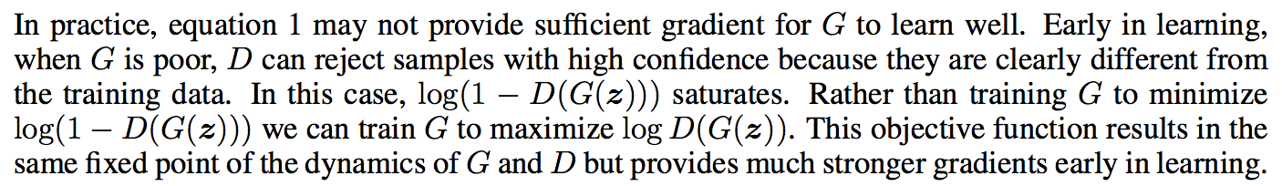
In our notation, this equals to the following alternative M-step:
$$
\theta_{t+1} \leftarrow \theta_t + \epsilon_t \frac{\partial}{\partial\theta} \mathbb{E}_{z\sim \mathcal{N}} \log D\left(G(z;\theta_t);\psi_{t+1}\right)
$$
In essence, we replaced $log(1-s)$ by $-log(s)$. These two functions are monotonically related, but have high gradients for different values of $s$. This nonlinear transformation allows the GAN algorithm to coneverge faster. (Well, sort of. When it does converge. It's still pretty unstable in my experience.)
As a result of this change, we don't really know what the algorithm minimises anymore. The connection to JS divergence is lost, and as far as I know, no-one has a good theoretical motivation for this alternative M-step objective.
Alternative M-step #2
Here, I'm going to talk about a third variant which can combines the alternative M-step above with the original M-step to obtain another meaningful update rule in the following form:
$$
\theta_{t+1} \leftarrow \theta_t + \epsilon_t \frac{\partial}{\partial\theta} \mathbb{E}_{z\sim \mathcal{N}} \log \frac{D\left(G(z;\theta_t);\psi_{t+1}\right)}{1 - D\left(G(z;\theta_t);\psi_{t+1}\right)}
$$
This is essentially just the sum of the updates in the first and second variants. What's interesting is that using this particular alternative step above, the GAN algorithm approximately minimises $\operatorname{KL}[Q|P]$ (see derivation below).
Also, we can assume the last operation of $D$ is applying a logistic sigmoid to transform its output to a valid probability between $0$ and $1$. The update above then simply corresponds to maximising the unnormalised classifier output, before it is fed into the sigmoid. This makes this output both very easy to calculate, and also quite intuitive to think about.
Connection to KL minimisation
To show that the alternative M-step above corresponds to minimising $KL[Q|P]$, one can turn to the same Bayes-optimal decision function argument one would use to show that the original GAN minimises JS divergence.
We know that for any generative model $Q$, the theoretical optimal discriminator between $P$ and $Q$ is given by this formula (assuming equal class priors):
$$
D^{*}(x) = \frac{P(x)}{P(x) + Q(x)}
$$
If assume that after the D-step, our discriminator $D$ is close to the Bayes-optimal $D^{*}$, the following approximation holds:
$$
\operatorname{KL}[Q|P] = \mathbb{E}_{x\sim Q} \log\frac{Q(x)}{P(x)}
$$
$$
= \mathbb{E}_{x\sim Q}\log\frac{1 - D^{\ast}(x)}{D^{\ast}(x)}
$$
$$
\approx \mathbb{E}_{x\sim Q}\log\frac{1 - D(x)}{D(x)}
$$
This is basically it, the image below shows what this variant of the algorithm does in practice on the Swiss roll toy example. It doesn't converge all the way in this animation, and possibly hyperparameters could be improved. The red contours show the real data distribution $P$ that we would like to model. The green dots show samples from the generative model, as training progresses. (each frame shows a subsequent $Q_t$ but with the hidden variable $z$ fixed throughout). The right-hand image shows the gradients of the objective function and how they change over time:
Connection to direct importance estimation
Using this presentation of the GAN algorithm we can reinterpret the goal of the D-step of GANs as a way to come up with an estimate to the log probability ratio $\log\frac{Q(x)}{P(x)}$ or $\log\frac{Q(x)}{Q(x) + P(x)}$ in order to minimise the KL or JS divergence. GANs happen to use a classifier to perform this estimation, but there are other ways to estimate these ratios directly from data.
There is a whole area of research on direct importance estimation or direct probability-ratio estimation which is looking at ways these probability ratios can be estimated from data samples. (see e.g. Sugiyama et al. 08; Kanamori 09).
Fitting a classifier using logistic regression and then extracting the unnormalised classifier as in "alternative M-step #2" has been one of the known ways to do this. (Qin, 1998; Cheng & Chu, 2004; Bickel et al., 2007). For more recent work, you can take a look at (Cranmer et al. 2016). But besides discriminative classifiers, you can use other algorithms based on kernels for example. The reason this connection between GANs and direct probability ratio estimation may not be immediately obvious is because these older papers cared primarily about the problem of domain adaptation, not so much about generative modelling.
In this context, one of the reasons GANs are so powerful is because they exploit convolutional neural networks, which we know work very well for representing images. However, we also know convnets are not-so-good with out-of-sample predictions, and they also tend to be pretty bad at representing the gradients of decision functions as evidenced by adversarial examples (Goodfellow et al. 2014). So I wonder if the combination of some aspects of GANs with other ways to estimate log-probability ratios can yield more stable generative modelling algorithms.
Final note on differential entropy
I just wanted to note that all these GAN related theories that rely on KL divergence or JS divergence have to be taken with a several sizeable pinches of salt and possibly a slice of lemon. GANs, by nature, generate a degenerate distribution that is concentrated on a nonlinear manifold, which is $0$-set in the space of all possible images. Therefore, unless this manifold of $Q$ lines up perfectly with the data generating distirbution $P$, all the arguments based on differential entropy and corresponding continuous KL divergences are a bit broken.
Even the Bayes-optimal classifier arguments underlying both the original Jensen-Shannon connection and my Kullback-Leibler connection are flawed. If $Q$ and $P$ are concentrated on different manifolds, the classification problem between them becomes trivial, and there are infinitely many classifiers achieving optimal Bayes risk, and the Jensen-Shannon divergence is always exactly 1 bit irrespective of parameters of $G$. The KL divergences are not even well defined in this case. The GAN idea still makes sense at a high level, partly because we limit the classifiers to functions that can be modelled by ConvNets, but it's probably important to keep this limitation of the theoretical analysis in mind.