How to Train your Generative Models? And why does Adversarial Training work so well?

One of the neat side-effects of maintaining a blog like this is that it forces me to write things down, allowing me to understand things better. This time I thought the ideas from my blog have become interesting enough for an ICLR submission which is now on arXiv:

• Ferenc Huszár (2015) How (not) to Train your Generative Model: Scheduled Sampling, Likelihood, Adversary? (under review for ICLR 2016)

The first part of this note is from an earlier post about why scheduled sampling is inconsistent. The second half I think is more interesting and talks generally about objective functions one should or should not use in generative modelling. This is not something I explained here before, so here we go.

Evaluating Generative Models

A key topic I'm very interested in is the choices of objective functions used in unsupervised learning and generative models. The key organising principle should be this: the objective function we use for training a probabilistic model should match the way we ultimately want to use the model. Yet, in unsupervised learning this is often overlooked and I think we lack clarity around what the models are used for and how they should be trained and evaluated. This paper tries to clarify this a bit in the context of generative models. I also want to mention that another ICLR submission this year also deals with this fundamental question: (Theis et al, 2016).

Here, I'm going to consider a narrow definition of generative models: models we actually want to use to generate samples from which are then shown to a human user/observer. This includes use-cases such as image captioning, texture generation, machine translation, speech synthesis and dialogue systems, but excludes things like unsupervised pre-training for supervised learning, semisupervised learning, data compression, denoising and many others. Very often people don't make this distinction clear when talking about generative models which is one of the reasons why there is still no clarity about what different objective functions do.

I argue that when the goal is to train a model that can generate natural-looking samples, maximum likelihood is not a desirable training objective. Maximum likelihood is consistent so it can learn any distribution if it is given infinite data and a perfect model class. However, under model misspecification and finite data (that is, in pretty much every practically interesting scenario), it has a tendency to produce models that overgeneralise.

KL divergence as a perceptual loss

Generative modelling is about finding a probabilistic model $Q$ that in some sense approximates the natural distribution of data $P$. When researchers (or users of their product) evaluate generative models for perceptual quality, they draw samples from it, then - for lack of a better word - eyeball the samples. In visual information processing this is often referred to as no-reference perceptual quality assessment \citep[see e.,g.\ ][]{wang2002noreference}. In the paper, I propose that the KL divergence $KL[Q| P]$ can be used as an idealised objective function to describe this scenario. This related to maximum likelihood which minimises $KL[P|Q]$, but different in fundamental ways which I will explain later.

Here is why I think $KL[Q|P]$ should be used: First, we can make the assumption that the perceived quality of each sample is related to the \emph{surprisal} $-\log Q_{human}(x)$ under the human observers' subjective prior of stimuli $Q_{human}(x)$. For those of you not familiar with computational cognitive science, this will seem ad-hoc, but it's a relatively common assumption to make when modelling reaction times in experiments for example. We further assume that the human observer maintains a very accurate model of natural stimuli, thus, $Q_{human}(x) \approx P(x)$. This is a fancy way of saying things like the observer being a native speaker therefore understanding all the nuances in language. These two assumptions suggest that in order to optimise our chances in this Turing test-like scenario, we need to minimise the following cross-entropy or perplexity term:

\begin{equation}
- \mathbb{E}_{x\sim Q} \log P(x)
\end{equation}

This perplexity is the exact opposite average negative log likelihood $- \mathbb{E}_{x\sim P} \log Q(x)$, with the role of $P$ and $Q$ changed. However, the perplexity alone would be maximised by a model $Q$ that deterministically picks the most likely stimulus. To enforce diversity one can simultaneously try to maximise the Shannon entropy of $Q$. This leaves us with the following KL divergence to optimise:

\begin{equation}
KL[Q| P] = - \mathbb{E}{x\sim Q} \log P(x) + \mathbb{E}{x\sim Q} \log Q(x)
\end{equation}

So if we want to train models that produce nice samples, my recommendation is to try to use $KL[Q|P]$ as an objective function or something that behaves like it. How does maximum likelihood compare?

Differences between maximum likelihood and $KL[Q|P]$

Maximum likelihood is roughly the same as minimising $KL[P|Q]$. The differences between minimising $KL[P|Q]$ and $K[Q|P]$ are well understood and it frequently comes up in the context of Bayesian approximate inference as well. Both divergences ensure consistency, minimising either converges to the true $P$ in the limit of infinite data and a perfect model class. However, they differ fundamentally in the way they deal with finite data and model misspecification (in almost every practical scenario):

• $KL[P|Q]$ tends to favour approximations $Q$ that overgeneralise $P$. If P is multimodal, the optimal $Q$ will tend to cover all the modes of $P$, even at the cost of introducing probability mass where $P$ has $0$ mass. Practically this means that the model will occasionally sample unplausible samples that don't look anything like samples from $P$.
• $KL[Q|P]$ tends to favour under-generalisation. The optimal $Q$ will typically describe the single largest mode of $P$ well, at the cost of ignoring other modes if they are hard to model without covering low-probability areas as well. Practically this means that $KL[Q|P]$ will try to avoid introducing unplausible samples, sometimes at the cost of missing the majority of plausible samples under $P$.

In other words: $KL[P|Q]$ is liberal, $KL[Q|P]$ is conservative. In yet other words: $KL[P|Q]$ is an optimist, $KL[Q|P]$ is a pessimist.

The problem of course is that $KL[Q|P]$ is super hard to optimise beased on a finite sample from $P$. Even harder than maximum likelihood. Not only that, the KL divergence is also not very well behaved, and is not well-defined unless $P$ is positive everywhere where $Q$ is positive. So there is little hope we can turn $KL[Q|P]$ into a practical training algorithm.

Generalised Adversarial Training

Generative Adversarial Networks(GANs) train a generative model jointly with an adversarial discriminative model that tries to differentiate between artificial and real data. The idea is, a generative model is good if it can fool the best discriminative model into thinking the generated samples are real. GANs have produced some of the nicest looking samples you'll find on the Internet and got people very excited about generative models again: human faces, album covers, etc.

How do they come into this picture? It's because they can be understood as approximately minimising the Jensen-Shannon divergence:

\begin{equation}
JSD[P|Q] = JSD[P|Q] = \frac{1}{2}KL\left[P\middle|\frac{P+Q}{2}\right] + \frac{1}{2}KL\left[Q\middle|\frac{P+Q}{2}\right].
\end{equation}

Looking at the equation above you can immediately see how it's related to this topic. JS divergence is a bit like a symmetrised version of KL divergence. It's not $KL[P|Q]$, not $KL[Q|P]$, but a bit of both. So one can expect that minimising JS divergence would exhibit a behaviour that is kind of halfway between the two extremes explained above. And that means that they would generate better samples than methods trained via maximum likelihood and similar objectives.

What's more, one can generalise JS divergence to a whole family of divergences, parametrised by a probability $0<\pi<1$ as follows:

\begin{equation}
JS_{\pi}[P|Q] = \pi \cdot KL[P|\pi P+(1-\pi)Q] + (1-\pi)KL[Q|\pi P+(1-\pi)Q].
\end{equation}

What I show in the paper is that by varrying $\pi$ between the two extremes, one can effectively interpolate between the behaviour of maximum likelihood ($\pi\rightarrow 0$) and minimising $KL[Q|P]$ ($\pi\rightarrow 1$). See the paper for details. This interpolation between behaviours is explained in this main figure below:

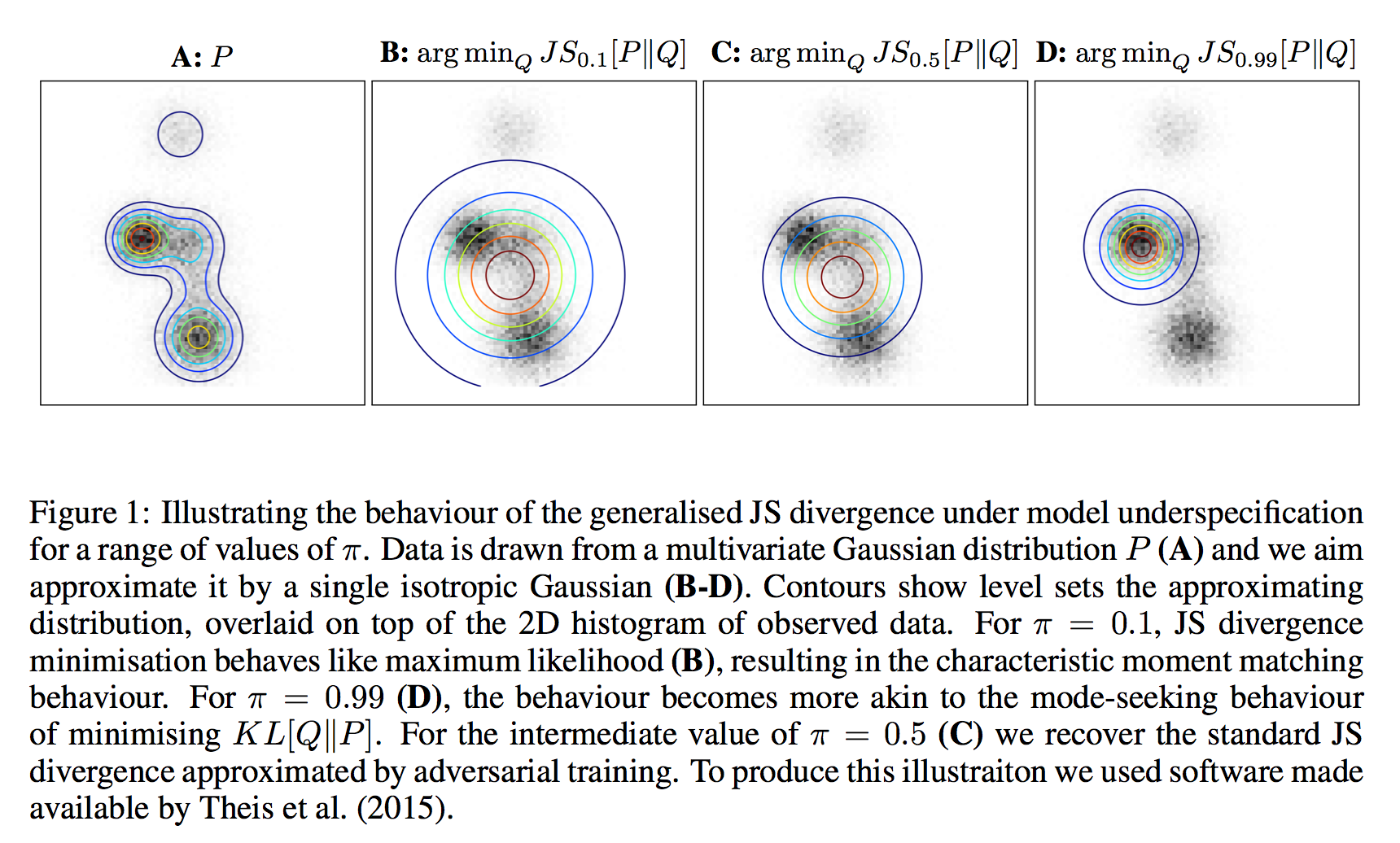
For any given value of $\pi$, we can optimise $JS_{\pi}$ approximately using an algorithm that is a slightly changed version of the original GAN algorithm. This is because the generalised JS divergence still has an elegant information theoretic interpretation. Consider a communications channel on which we can transmit a single data point of some kind. We toss a coin and with probability $\pi$, we send a sample from $P$, and with probability $1-\pi$ we send a sample from $Q$ instead. The receiver doesn't know the outcome of the coinflip, she only observes the sample. The $JS_{\pi}$ is the mutual information between the observed sample and the coinflip. It is also an upper bound on how well any algorithm can do in guessing the coinflip from the observed sample.

To implement an adversarial training algorithm for $JS_{\pi}$ one simply needs to change the ratio of samples the discriminative network sees from $Q$ vs $P$ (or apply appropriate weights during training). In the original method the discriminator network is faced with a balanced classification problem, i.e. $\pi=\frac{1}{2}$. It is hard to believe, but this irrelevant-looking modification changes the behaviour of the GAN algorithm dramatically, and can in theory allow the GAN algorithm to approximate both maximum likelihood or $KL[Q|P]$.

This analysis explains why GANs have been so successful in generating very nice looking images, and relatively few weird-looking ones. It is also worth pointing out that the GAN method is still in its infantcy and has many issues and limitations. The main issue is that it is based on sampling from $Q$ which doesn't work well in high dimensions. Hopefully some of these limitations can be overcome and then we should have a pretty powerful framework for training good generative models.