Understanding Minibatch Discrimination in GANs
Yesterday I read the latest paper by the OpenAI folks on practical tricks to make GAN traning stable:
- Tim Salimans, Ian Goodfellow, Wojciech Zaremba, Vicki Cheung, Alec Radford, Xi Chen (2016) Improved Techniques for Training GANs
There was one idea in there which got me thinking, and this is what I wanted to write about here: minibatch discrimination.
Summary of this post
- How does this minibatch discrimination heuristic work and how does it change the behaviour of the GAN algorithm? Does it change the underlying objective function that is being minimized?
- the answer is: for the original GAN algorithm that minimises Jensen-Shannon divergence it does change the behaviour in a non-trivial way. One side-effect is assigning a higher relative penalty for low-entropy generators.
- when using the blended update rule from here, the algorithm minimises the reverse KL-divergence. In this case, using minibatch discrimination leaves the underlying objective unchanged: the algorithm can still be shown to miminise KL divergence.
- even if the underlying objectives remain the same, using minibatch discrimination may be a very good idea practically. It may stabilise the algorithm by, for example, providing a lower variance estimator to log-probability-ratios.
Here is the ipython/jupyter notebook I used to draw the plots and test some of the things in this post in practice.
What is minibatch discrimination?
In the vanilla Generative Adversarial Networks (GAN) algorithm, a discriminator is trained to tell apart generated synthetic examples from real data. One way GAN training can fail is to massively undershoot the entropy of the data-generating distribution, and concentrate all it's parameters on generating just a single or few examples.
To remedy this, the authors play with the idea of discriminating between whole minibatches of samples, rather than between individual samples. If the generator has low entropy, much lower than real data, it may be easier to detect this with a discriminator that sees multiple samples.
Here, I'm going to look at this technique in general: modifying an unsupervised learning algorithm by replacing individual samples with i.i.d. minibatches of samples. Note, that this is not exactly what the authors end up doing in the paper referenced above, but it's an interesting trick to think about.
How does the minibatch heuristic effect divergences?
The reason I'm so keen on studying GANs is the connection to principled information theoretic divergence criteria. Under some assumptions, it can be shown that GANs minimise the Jensen-Shannon (JS) divergence, or with a slight modification the reverse-KL divergence. In fact, a recent paper showed that you can use GAN-like algorithms to minimise any $f$-divergence.
So my immediate question looking at the minibatch discrimination idea was: how does this heuristic change the divergences that GANs minimise.
KL divergence
Let's assume we have any algorithm (GAN or anything else) that minimises KL divergence $\operatorname{KL}[P|Q]$ between two distributions $P$ and $Q$. Let's now modify this algorithm so that instead of looking at distributions $P$ and $Q$ of a single sample $x$, it looks at distributions $P^{(N)}$ and $Q^{(N)}$ of whole a minibatch $(x_1,\ldots,x_N)$. I use $P^{(N)}$ to denote the following distribution:
$$
P^{(N)}(x_1,\ldots,x_N) = \prod_{n=1}^N P(x_n)
$$
The resulting algorithm will therefore minimise the following divergence:
$$
d[P|Q] = \operatorname{KL}[P^{(N)}|Q^{(N)}]
$$
It is relatively easy to show why this divergence $d$ behaves exactly like the KL divergence between $P$ and $Q$. Here's the maths for minibatch size of $N=2$:
\begin{align}
d[P|Q] &= \operatorname{KL}[P^{(2)}|Q^{(2)}] \\
&= \mathbb{E}_{x_1\sim P,x_2\sim P}\log\frac{P(x_1)P(x_2)}{Q(x_1)Q(x_2)} \\
&= \mathbb{E}_{x_1\sim P,x_2\sim P}\log\frac{P(x_1)}{Q(x_1)} + \mathbb{E}_{x_1\sim P,x_2\sim P}\log\frac{P(x_2)}{Q(x_2)} \\
&= \mathbb{E}_{x_1\sim P}\log\frac{P(x_1)}{Q(x_1)} + \mathbb{E}_{x_2\sim P}\log\frac{P(x_2)}{Q(x_2)} \\
&= 2\operatorname{KL}[P|Q]
\end{align}
In full generality we can say that:
$$
\operatorname{KL}[P^{(N)}|Q^{(N)}] = N \operatorname{KL}[P|Q]
$$
So changing the KL-divergence to minibatch KL-divergence does not change the objective of the training algorithm at all. Thus, if one uses minibatch discrimination with the blended training objective, one can rest assured that the algorithm still performs approximate gradient descent on the KL divergence. It may still work differently in practice, for example by reducing the variance of the estimators involved.
This property of the KL divergence is not surprising if one considers its compression/information theoretic definition: the extra bits needed to compress data drawn from $P$, using model $Q$. Compressing a minibatch of i.i.d. samples corresponds to compressing the samples independently. Their codelengths would add up linearly, hence KL-divergences add up linearly, too.
JS divergence
The same thing does not hold for the JS-divergence. Generally speaking, minibatch JS divergence behaves differently from ordinary JS-divergence. Instead of equality, for JS divergences the following inequality holds:
$$
JS[P^{(N)}|Q^{(N)}] \leq N \cdot JS[P|Q]
$$
In fact for fixed $P$ and $Q$, $JS[P^{(N)}|Q^{(N)}]/N$ is monotonically non-increasing. This can be seen intuitively by considering the definition of JS divergence as the mutual information between the samples and the binary indicator $y$ of whether the samples were drawn from $Q$ or $P$. Using this we have that:
\begin{align}
\operatorname{JS}[P^{(2)}|Q^{(2)}] &= \mathbb{I}[y ; x_1, x_2] \\
&= \mathbb{I}[y ; x_1] + \mathbb{I}[y ; x_2 \vert x_1] \\
&\leq \mathbb{I}[y ; x_1] + \mathbb{I}[y ; x_2] \\
&= 2 \operatorname{JS}[P|Q]
\end{align}
Below I plotted the minibatch-JS-divergence $JS[P^{(N)}|Q^{(N)}]$ for various minibatch-sizes $N=1,2,3,8$, between univariate Bernoulli distributions with parameters $p$ and $q$. For the plots below, $p$ is kept fixed at $p=0.2$, and the parameter $q$ is varied between $0$ and $1$.
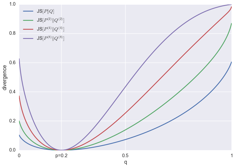
You can see that all divergences have a unique global minimum around $p=q=0.2$. However, their behaviour at the tails changes as the minibatch-size increases. This change in behaviour is due to saturation: JS divergence is upper bounded by $1$, which corresponds to 1 bit of information. If I continued increasing the minibatch-size (which would blow up the memory footprint of my super-naive script), eventually the divergence would reach $1$ almost everywhere except for a dip down to $0$ around $p=q=0.2$.
Below are the same divergences normalised to be roughly the same scale.

The problem of GANs that minibatch discrimination was meant to fix is that it favours low-entropy solutions. In this plot, this would correspond to the $q<0.1$ regime. You can argue that as the batch-size increases, the relative penalty for low-entropy approximations $q<0.1$ do indeed decrease when compared to completely wrong solutions $q>0.5$. However, the effect is pretty subtle.
Bonus track: adversarial preference loss
In this context, I also revisited the adversarial preference loss. Here, the discriminator receives two inputs $x_1$ and $x_2$ (one synthetic, one real) and it has to decide which one was real.
This algorithm, too, can be related to the minibatch discrimination approach, as it minimises the following divergence:
$$
d(P,Q) = d(P\times Q|Q\times P),
$$
where $P\times Q(x_1,x_2) = P(x_1)Q(x_2)$. Again, if $d$ is the $KL$ divergence, the training objective boils down to the same thing as the original GAN. However, if $d$ is the JS divergence, we will end up minimising something weird, $\operatorname{JS}[Q\times P| P\times Q]$.