The Spherical Kernel Divergence

This post is about an interesting kernel-based divergence measure I found when I wrote up my thesis on scoring rules and divergences in machine learning. It's been largely forgotten, I'm not aware of this being discussed elsewhere. I thought I'll put it out here in case people find it useful.

Background

Scoring rules and divergences

Scoring rules are best described in terms of forecasting: Let's assume we want to forecast some - so far unobserved - quantity $x$. We can summarise our forecast as a probability distribution $Q$ over possible outcomes. A scoring rule $S(x,Q)$ assigns a penalty to our probabilistic forecast $Q$ in the light of the actual observation $x$.

A common scoring rule in machine learning is the log loss: $S_{\log}(x,Q) = - \log Q(x)$. When one does maximum likelihood training of $Q$, that boils down to minimising the expected score $\operatorname{argmin}_\theta \mathbb{E}_{x\sim P}S_{\log}(x,Q_\theta)$. But the logarithmic is just one of many useful examples of scoring rules.

Based on a scoring rule $S$ one can define a divergence, which, under some conditions, is a Bregman divergence:

$$
d_S(P,Q) = \mathbb{E}_{x\sim P}S(x,Q) - \mathbb{E}_{x\sim P}S(x,P)
$$

The scoring rule is called strictly proper, and the corresponding divergence a Bregman divergence, if and only if the following holds:

$$
d(P,Q)=0 \iff P=Q
$$

So strictly proper scoring rules are useful, because minimising the average score over some dataset allows us to consistently recover the true data distribution $P$, as long as our model class $Q$ contains $P$.

For the logarithmic score, the corresponding divergence is the KL-divergence

$$
\operatorname{KL}[P|Q] = \mathbb{E}_{x\sim P}\log\frac{P(x)}{Q(x)}
$$

There are many other useful scoring rules, and corresponding divergences, for a review see (Gneiting & Raftery, 2007) or chapter 1 of my thesis.

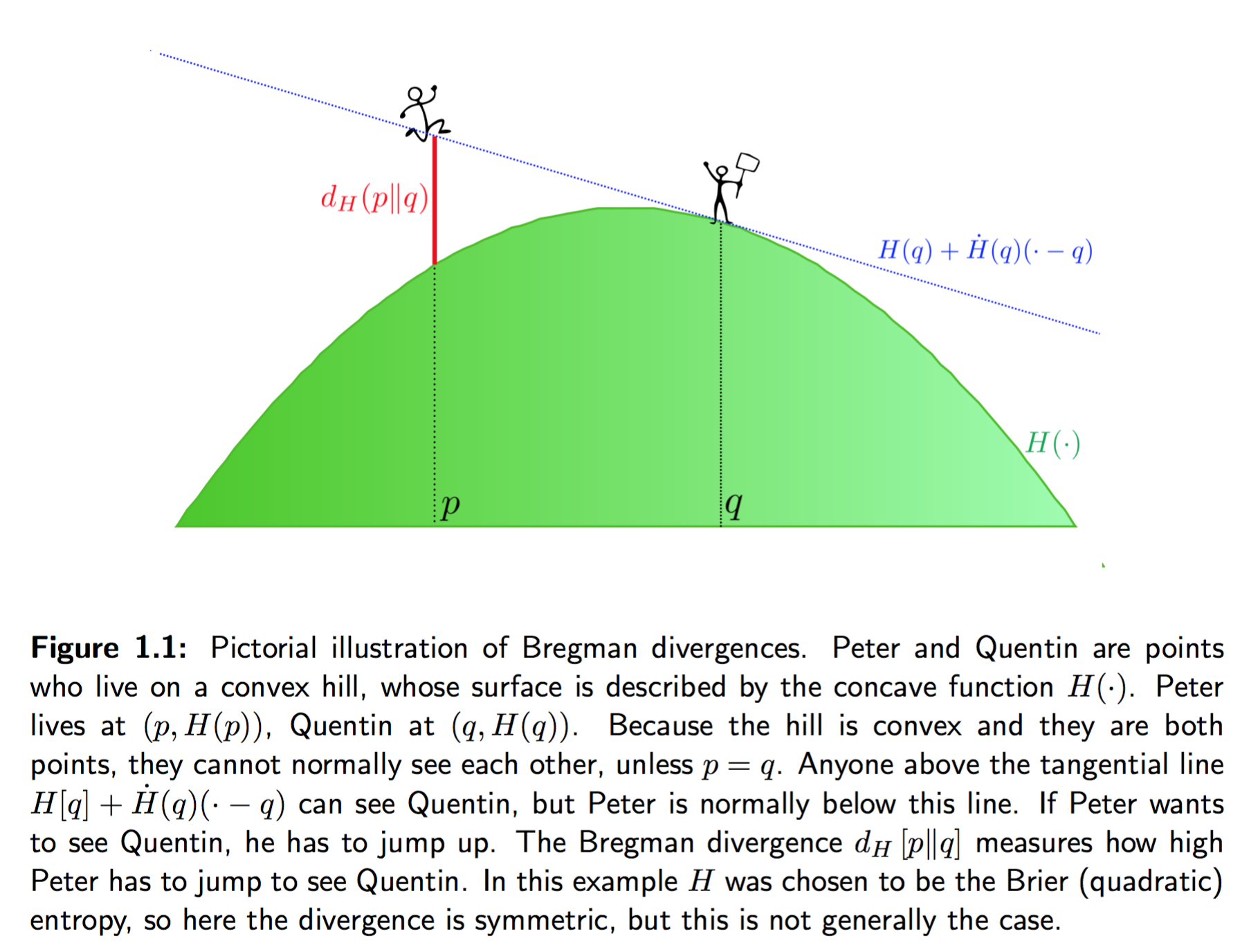
Finally, here is a lighthearted, graphical illustration of Bregman divergences, in terms of the entropy function $\mathbb{H}_S[Q] = \mathbb{E}_{x\sim Q}S(x,Q)$:

Maximum mean discrepancy and the kernel scoring rule

I'm going to show another divergence, maximum mean discrepancy (MMD), and the associated kernel scoring rule. MMD is used in two-sample testing, and more recently in Generative Moment Matching Networks (Li et al, (2016), Dziugaite et al. (2016)) for generative modelling.

\begin{align}
\operatorname{MMD}^2(x,y) &= \sup_{|f|_{\mathcal{H}_k}=1} \left( \mathbb{E}_{x\sim P}f(x) - \mathbb{E}_{x\sim Q}f(x) \right)^2\\
&= |\mu_P - \mu_Q|_{\mathcal{H}_k}^2\\
&= \mathbb{E}_{x,y\sim P} k(x,y) + \mathbb{E}_{x,y\sim Q} k(x,y) - 2 \mathbb{E}_{x\sim P,y\sim Q} k(x,y)
\end{align}

The first line explains why this divergence is called Maximum Mean Discrepancy: it finds the worst-case function $f$ (from the unit ball of the Hilbert-space, $|f|_{\mathcal{H}_k}=1$) whose average value under $P$ is most different from its average under $Q$. In this sense, $f$ plays a similar role to the adversarial discriminator in GANs: it's trying to characterise the differences between $P$ and $Q$.

The second line is the definition in terms of the so called mean embeddings: the functions $\mu_P = \mathbb{E}_{x\sim P}k(\cdot,x)$ and $\mu_Q = \mathbb{E}_{x\sim Q}k(\cdot,x)$ in the Hilbert space which uniquely characterise $P$ and $Q$, respectively.

The third line expresses MMD in terms of the kernel function $k$, and this is the formula we use when we actually want to compute this divergence.

The squared MMD is in fact a Bregman divergernce which corresponds to the kernel scoring rule, defined as follows:

\begin{align}
S_k(x,Q) &= k(x,x) - 2\mathbb{E}_{y\sim Q}k(x,y) + \mathbb{E}_{y,z\sim Q}k(y,z)\\
&= \sup_{|f|_{\mathcal{H}_k}=1} (f(x) - \mathbb{E}_{y\sim Q} f(y))^2\\
&= |k(\cdot,x) - \mu_Q|_{\mathcal{H}_k}^2\\
&= MMD^2(\delta_x, Q)
\end{align}

What is interesting about this scoring rule is that you can view it as the kernel generalisation of the ancient Brier scoring rule (Brier, 1950. Gneiting & Raftery, 2017) which measures $L_2$ norm rather than RKHS-norm:

\begin{align}
S_{Brier}(x,Q)&= |\delta_x - Q |_2^2\\
&= |Q|_2^2 - 2Q(x) + 1
\end{align}

Where $|Q|_2$ is the $L_2$-norm of $Q$ defined as $|Q|_2 = \sqrt{\mathbb{E}_{y\sim Q}Q(y)}$. The Brier score can be viewed as the kernel score with an extremely narrow kernel: $k(x,y)\rightarrow \delta(x-y)$.

The spherical kernel score

And this brings us to the actual meat in this post. The Brier score has a younger sister, called the spherical score (Good, 1971.Gneiting & Raftery, 2017):

\begin{align}
S_{spherical}(x,Q) &= 1 - \frac{Q(x)}{|Q|_2} \\
&= 1 - \frac{Q(x)}{\sqrt{\mathbb{E}_{y\sim Q}Q(y)}}
\end{align}

The question arises, if the Brier/quadratic divergence has a kernel analog in MMD, can we also construct a kernel analog to the spherical score and its divergence? The answer is yes, and this is what I call the spherical kernel score.

\begin{align}
S_{spherical,k}(x,Q) &= 1 - \frac{\mu_Q(x)}{|\mu_Q|_{\mathcal{H}_k}|\mu_{\delta_x}|_{\mathcal{H}_k}} \\
&= 1 - \frac{\mathbb{E}_{y\sim Q}k(x,y)}{\sqrt{k(x,x)\mathbb{E}_{y,z\sim Q}k(y,z)}}
\end{align}

And the associated divergence, which I call spherical kernel divergence (SKD, $d_{spherical,k}$) becomes:

\begin{align}
d_{spherical,k}(P,Q) &= 1 - \frac{\langle\mu_P,\mu_Q\rangle_{\mathcal{H}_k}}{|\mu_Q|_{\mathcal{H}_k}|\mu_P|_{\mathcal{H}_k}}\\
&= 1 - \cos(\mu_P,\mu_Q)\\
& = 1 - \frac{\mathbb{E}_{x\sim P,y\sim Q}k(x,y)}{\sqrt{\mathbb{E}_{x,y\sim P}k(x,y)\mathbb{E}_{x,y\sim Q}k(x,y)}},
\end{align}

where $\langle\mu_P,\mu_Q\rangle_{\mathcal{H}_k}$ denotes inner product between the mean embeddings and $\cos(\mu_P,\mu_Q)$ is defined as

$$
\cos(\mu_P,\mu_Q) = \frac{\langle\mu_P,\mu_Q\rangle_{\mathcal{H}_k}}{|\mu_P|_{\mathcal{H}_k}|\mu_Q|_{\mathcal{H}_k}}.
$$

While MMD measures the analog of Euclidean distance between mean embeddings, the spherical kernel divergence measures the analog of cosine dissimilarity between them. Just as with MMD and the Brier divergence, the spherical kernel score reduces to the spherical score in the limit of infinitesimal kernel bandwidth $k(x,y)\rightarrow \delta(x-y)$.

Random projections interpretation

There is an interesting property of cosine dissimilarity, which is used to approximate cosine distance via locality sensitive hashing (LSH). This allows us to interpret the SKD as follows:

\begin{align}
d_{spherical,k}(P,Q) &= \mathbb{P}_{f\sim \mathcal{GP}_k} \left[ \operatorname{sign}(\langle f,\mu_P \rangle) \neq \operatorname{sign}(\langle f,\mu_P \rangle) \right]\\
&= \mathbb{P}_{f\sim \mathcal{GP}_k} \left[ \operatorname{sign}(\mathbb{E}_{x\sim P}f(x)) \neq \operatorname{sign}(\mathbb{E}_{x\sim Q}f(x))\right]
\end{align}

So, let's say we sample a bunch of smooth scalar test functions $f$ from a Gaussian process with covariance kernel $k$. We take the average of each test function on samples from $P$ as well as on samples from $Q$. Then we take the average of each test function under $P$ and under $Q$ and we look at the probability that the signs differ. So while the MMD cares about the squared difference between $\mathbb{E}_{x\sim P}f(x)$ and $\mathbb{E}_{x\sim Q}f(x)$, the SKD only cares about whether they have the same the same sign or not.

As $f$ are drawn from a Gaussian Process, $\mathbb{E}_{x\sim P}f(x)$ and $\mathbb{E}_{x\sim Q}f(x)$ are jointly Gaussian distributed, with mean $0$ and covariance that depends on $P$ and $Q$ as well as the kernel $k$. Below is a toy figure of such 2D Gaussian, and I shaded the areas where the sign of $\mathbb{E}_{P}f$ and \mathbb{E}_{Q}f$ match. Obviously, the more positively correlated the two random variables are, the higher percentage of probability mass is placed here:

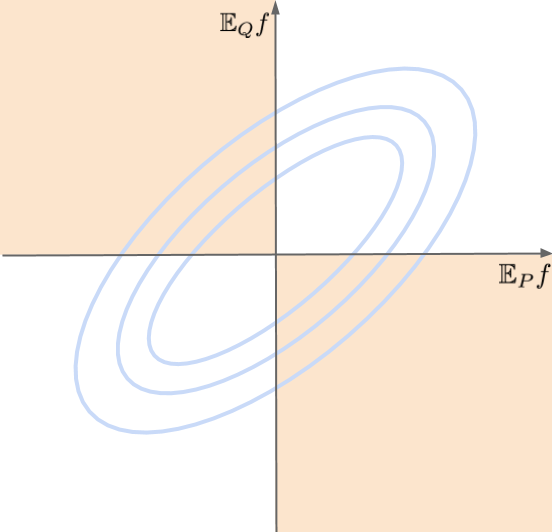
Compare this with the MMD which tries to minimise the average squared difference between $\mathbb{E}_{x\sim P}f(x)$ and $\mathbb{E}_{x\sim Q}f(x)$. Both divergences will try to push this Gaussian to be a perfectly correlated, they just differ in how exactly they do it.

If you want to play around with these formulae a little bit more, as homework, try to work exactly what these covariances are (not very hard), and express the spherical kernel score in terms of quadrant probabilities of bivariate normal distributions.

Summary and questions

In this post I've (re)introduced the spherical kernel divergence and an associated strictly proper scoring rule for comparing probability distributions. It is related to maximum mean discrepancy, but instead of squared RKHS-distance it measures the cosine distance between the kernel mean embeddings of the two distributions.

Why is this even useful?

Not sure. Not sure it's even useful, but I think it's interesting to think about different divergences one can define based on kernel Hilbert spaces. Unlike MMD, the spherical kernel score is scale independent, in the sense that the value of the divergence remains the same if we multiply either $Q$ or $P$ distributions by a scalar. So technically, the spherical divergence can be computed between two distributions whose normalising constants are intractable. Of course one still has calculate integrals of the form $\int \int P(x) k(x,y) Q(z) dz dx$ and $\int \int Q(x) k(x,y) Q(z) dz dx$ up to a constant. So whether or not this property can be turned into something useful remains to be seen.

Another thing I'm looking for is an ability to optimise the kernel hyperparameters in the divergence. For the MMD this is hard, although there is promising recent progress (Sutherland et al. 2016). Maybe SKD can unlock new ways in which optimising $k$ can be achieved.

Outstanding challenges

The obvious question is: How can we approximate the spherical kernel score in an unbiased way, from finite samples? This is a requirement if we want to use it for generative modelling - if we want to do stochastic gradient descent. BTW, hat tip to Dziugaite et al. (2016) who actually used the unbiased MMD estimate in their version of generative moment matching networks (Eq. (8)) , while Li et al, (2016) used a biased estimate (Eqn. (3)). I don't actually know what an unbiased estimate of the spherical kernel divergence would look like, so if you do, please leave a comment!