Pruning Neural Networks: Two Recent Papers

I wanted to briefly highlight two recent papers on pruning neural networks (disclaimer, one of them is ours):

• Christos Louizos, Max Welling, Diederik P. Kingma (2018) Learning Sparse Neural Networks through $L_0$ Regularization
• Lucas Theis, Iryna Korshunova, Alykhan Tejani, Ferenc Huszár (2018) Faster gaze prediction with dense networks and Fisher pruning

What I generally refer to as pruning in the title of this post is reducing or controlling the number of non-zero parameters, or the number of featuremaps actively used in a neural network. At a high level, there are at least three ways one can go about this, pruning is really only one of them:

• regularization modifies the objective function/learning problem so the optimization is likely to find a neural network with small number of parameters. Louizos et al, (2018) choose this approach.
• pruning takes a large network and deletes features or parameters that are in some sense redundant (Theis et al, 2018) is an example of this
• growing: although less wide-spread you can take a third approach where, starting from a small network, you incrementally add new units by some growth criterion

Why do this?

There are different reasons for pruning your network. The most obvious, perhaps, is to reduce computational cost while keeping the same performance. Removing features which aren't really used in your deep network architecture can speed up inference as well as training. You can think also think of pruning as a form of architecture search: figuring out how many features you need in each layer for best performance.

The second argument is to improve generalization by reducing the number of parameters, and thus the redundancy in the parameter space. As we have seen in recent work on generalization in deep networks, the raw number of parameters ($L_0$ norm) is not actually a sufficient predictor of their generalization ability. That said, we empirically find that pruning a network tends to help generalization. Meanwhile, the community is developing (or, putting my Schmidhuber-hat on: maybe in some cases rediscovering) new parameter-dependent quantities to predict/describe generalization. The Fisher-Rao norm is a great example of these. Interestingly, Fisher pruning (Theis et al, 2018) turns out to have a nice connection to the Fisher-Rao norm, and this may hint at a deeper relationship between pruning, parameter redundancy and generalization.

$L_0$ regularization

I found the $L_0$ paper by Louizos et al, (2018) very interesting in that it can be seen as a straightforward application of the machine learning problem transformations I wrote up in the machine learning cookbook a few months ago. It's a good illustration of how you can use these general ideas go from formulating an intractable ML optimization problem to something practical you can run SGD on.

So I will summarize the paper as a series of steps, each changing the optimization problem:

1. start from an ideal loss function which may be intractable to optimize: the usual training loss plus the $L_0$ norm of parameters, combined linearly. The $L_0$ norm simply counts non-zero entries in a vector, a non-differentiable piecewise constant function. This is a difficult, combinatorial optimization problem.
2. apply variational optimization to turn the non-differentiable function into a differentiable one. This generally works by introducing a probability distribution $p_{\psi}(\theta)$ over parameters $\theta$. Even if the objective is non-differentiable with respect to any $\theta$, the average loss under $p_{\psi}$ may be differentiable w.r.t. $\psi$. To find the optimal $\psi$, one can generally use a REINFORCE gradient estimator, which results in evolution strategies. But ES generally has very high variance, so we
3. apply the reparametrization trick to $p_\psi$ to construct a lower-variance gradient estimator. This, however, only works for continuous variables. To deal with the discreteness, we turn to a
4. concrete relaxation, which approximates the discrate random variable by a continuous approximation. Now we have a lower-variance (compared to REINFORCE) gradient estimator which one can calculate via backprop and simple Monte Carlo sampling. You can use these gradients in SGD (Adam), which is what the paper does.

Interestingly, the connection between Eq. (3) and evolution strategies or variational optimization is not mentioned. Instead, a motivation based on a different connection to spike-and-slab priors is given. I recommend reading the paper, perhaps with this connection in mind.

The authors then show that this indeed works, and compares favourably to other methods designed to reduce the number of parameters.
Thinking about the paper in terms of these steps converting from one problem to another allows you to generalize or improve the idea. For example, the REBAR or RELAX gradient estimators provide an unbiased and lower-variance alternative to the concrete relaxation, which may work very well here, too.

Fisher pruning

The second paper I wanted to talk about is something from our own lab. Rather than being a purely methods paper, (Theis et al, 2018) focusses on the specific application of building speedy neural networks to predict saliency in an image. The pruned network now powers the logic behind cropping photos on Twitter.

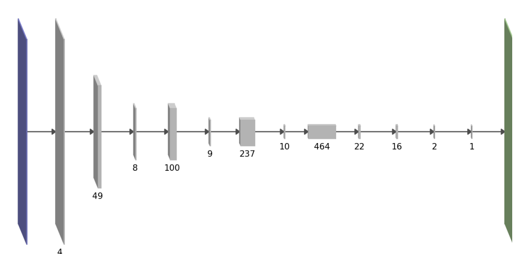
Our goal, too, was to reduce computational cost of the network, and specifically in the transfer learning setting: when building on top of a pre-trained neural network, you inherit a lot of complexity required to solve the original source task, much of which may be redundant for solving your target task. There is a difference in our high-level pruning objective: unlike $L_0$ norm or group sparsity, we used a slightly more complicated formula to directly estimates the forward pass runtime of the method. This is a quadratic function of the number of parameters at each layer with interactions between neighbouring layers. Interestingly, this results in architectures which tend to alternate thick and thin layers, like the one below:

We prune the trained network greedily by removing convolutional featuremaps one at a time. A meaningful principle for selecting the next feature map to prune is to minimize the resulting increase in training loss. Starting from this criterion, using a second order Taylor-expansion of the loss, making some more assumptions, we obtain the following pruning signal for keeping a parameter $\theta_i$:

$$
\Delta_i \propto F_i \theta_i^2,
$$

where $F_i$ denotes the $i^{th}$ diagonal entry of the Fisher information matrix. The above formula deals with removing a single parameter, but we can generalize this to removing entire featuremaps. Pruning proceeds by removing the parameter or featuremap with the smallest $\Delta$ in each iteration, and retraining the network between iterations. For more details, please see the paper.

Adding to what's presented in the paper, I wanted to point out a few connections between Fisher pruning to ideas I discussed on this blog before.

Fisher-Rao norm

The first connection is to the Fisher-Rao norm. Assume for a minute that the Fisher information is diagonal - a big and unreasonable assumption in theory, but a pragmatic simplification resulting in useful algorithms in practice. With this assumption, the Fisher-Rao norm of $\theta$ becomes:

$$
|\theta|_{fr} = \sum_{i=1}^{I} F_i \theta_i^2
$$

Written in this form, you can hopefully see the connection between the FR-norm and the Fisher pruning criterion. Depending on the particular definition of Fisher information used, you can interpret the FR-norm, approximately, as

• the expected drop in training log likelihood (empirical Fisher Info) as you remove a random parameter, or as
• the approximate change in the conditional distribution defined by the model (model Fisher info) as we remove a parameter

In the real world, the Fisher info matrix is not diagonal, and this is actually an important aspect of understanding generalization. For one, considering only diagonal entries makes Fisher pruning sensitive to certain reparametrizations (ones with non-diagonal Jacobian) of the network. But maybe there is a deeper connection to be observed here between Fisher-Rao norms and the redundancy of parameters.

Elastic Weight Consolidation

Using the diagonal Fisher information values to guide pruning also bears resemblance to elastic weight consolidation by (Kirkpatrick et al, 2017). In EWC, the Fisher information values are used to establish which weights are more or less important for solving previous tasks. There, the algorithm was derived from the perspective Bayesian on-line learning, but you can also motivate it from a Taylor expansion perspective just like Fisher pruning.

The metaphor I use to understand and explain EWC is that of a shared hard drive. (WARNING: like all metaphors, this may be completely missing the point). The parameters of a neural network are like a hard drive or storage volume of some sort. Training the NN on a task involves compressing the training data and saving the information to the hard drive. If you have no mechanism to keep data from being overwritten, it's going to be overwritten: in neural networks, catastrophic forgetting occurs the same way. EWC is like a protocol for sharing the hard-drive between multiple users, without the users overwriting each other's data. The Fisher information values in EWC can be seen as soft do-not-overwrite flags. After training on the first task, we calculate the Fisher information values which say which parameters store crucial information for the task. The ones with low Fisher value are redundant and can be reused to store new info. In this metaphor, it is satisfying to think about the sum of Fisher information values as measuring how full the hard-drive is, and pruning as throwing away parts of the drive not actually used to store anything.

Summary

I wrote about two recent methods for automatically learning neural network architecture by figuring out which parameters/features to throw away. In my mind, both methods/papers are interesting in their own right. The $L_0$ approach seems like a simpler optimization algorithm that may be preferable to the iterative, remove-one-feature-at-a-time nature of Fisher pruning. However, Fisher pruning is more applicable to the scenario when you start from a large pretrained model in a transfer learning setting.