Notes on the Limitations of the Empirical Fisher Approximation
This post is a short not on an excellent recent paper on empirical Fisher information matrices:
- Kunstner, Balles and Hennig (2019) Limitations of the Empirical Fisher Approximation
I was debating with myself whether I should write a post about this because it's a superbly written paper that you should probably read in full. There isn't a whole lot of novelty in the paper, but it is a great discussion paper that provides a concise overview of the Fisher information, the empirical Fisher matrix and their connectinos to generalized Gauss-Newton methods. For more detail, I also recomend this older and longer overview by James Martens.
The Fisher and the empirical Fisher
For a supervised learning model $p_\theta (y\vert x)$ the Fisher infromation matrix for a specific input $x$ is defined as follows:
$$
F_x = \mathbb{E}_{p_\theta(y\vert x)} \left[ \nabla_\theta \log p_\theta(y\vert x) \nabla_\theta \log p_\theta(y\vert x)^\top \right]
$$
The Fisher information roughly measures the sensitivity of the model's output distribution to small changes in the parameters $\theta$. For me, the most intuitive interpretation is that it is the local curvature $KL[p_\theta\vert p_{\theta'}]$ as $\theta' \rightarrow \theta$. So, by using the Fisher infromation as a quadratic penalty, or as a preconditioner in second order gradient descent, you're penalizing changes to the model's output distribution as measured by the KL divergence. This makes sense especially for neural networks, where small changes in network parameters can lead to arbitrary changes in the function the model actually implements.
If you have an entire distribution or a dataset, you normally add up the pointwise $F_x$ matrices to form the Fisher information for the whole training data:
$$
F = \sum_n F_{x_n} = \sum_n \mathbb{E}_{p_\theta(y\vert x_n)} \left[ \nabla_\theta \log p_\theta(y\vert x_n) \nabla_\theta \log p_\theta(y\vert x_n)^\top \right]
$$
In pracice, however, people often work with another matrix instead, which is called the empirical Fisher information matrix, defined as follows:
$$
\tilde{F} = \sum_n\left[ \nabla_\theta \log p_\theta(y_n\vert x_n) \nabla_\theta \log p_\theta(y_n\vert x_n)^\top \right]
$$
The difference, of course, is that rather than sampling $y$ from the model itself, here, we use the observed labels $y_n$ from the dataset. This matrix, while it's often used, does not have a principled motivation. The paper shows how it lacks most properties that make the Fisher information so useful quantity in many cases, and it also lacks any principled motivation. The paper's simple, yet insightful, examples show how using the empirical Fisher instead of the real Fisher in second order optimization can lead to bonkers results:
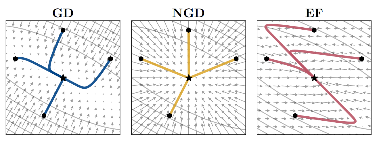
What the above example shows is the vector field corresponding to differently preconditioned gradient descent algorithms in a two-parameter simple least squares linear regresesion example. The first panel shows the gradients field. The second shows the natural graident field, i.e. gradients corrected by the inverse Fisher information. The third shows the gradients corrected by the empirical Fisher instead. You can see that the empirical Fisher does not make the optimization problem any easier or better conditioned. The bottom line is: you probably shouldn't use it.
But aren't they the same near the minimum?
One particular myth that Kunstner et al (2019) try to debunk is that the Fisher and empirical Fisher coincide near minima of the loss function, and therefore either can be safely usef once you're done with training your model. I have made this argument several times in the past myself. If you look at he definitions, it's easy to conclude that they should indeed coincide under two conditions:
- that the model $p_\theta(y\vert x)$ closely approximates the true sampling distribution $p_\mathcal{D}(y\vert x)$, and
- that you have sufficiently large $N$ (number of samples) so that both the Fisher and empirical Fisher converge to their respective population average.
The paper argues that these two conditions are often at odds in practice. One either uses a simple model, in which case model misspecification is likely, meaning $p_\theta(y\vert x)$ can't approximate the true underlying $p_\mathcal{D}(y\vert x)$ well. Or, one uses an expressive, overparametrised model, such as a big neural network, in which case some form of overfitting likely happens, and $N$ is too small for the two matrices to coincide. The paper offers a lot more nuance to this, and again, I highly recommend reading it whole.
Direction of preconditioned gradients
The paper also looks at comparing the direction of the natural gradient with the empirical Fisher-corrected gradients, and finds that the EF gradient often tries to go in a very different direction than the natural gradient.
It's also interesting to look at the projection of the EF gradient onto the original gradient, to see how big an EF-gradient update is in the direction of normal gradient descent.
The gradient for a single datapoint $(x_n, y_n)$ is g_n = -\nabla_\theta \log p_\theta(y_n\vert x_n). If we use the EF matrix as preconditioner, the gradient is modifierd to $\tilde{g}_n = \tilde{F}^{-1}g_n = -\tilde{F}^{-1} \nabla_\theta \log p_\theta(y_n\vert x_n)$. Let's look at the inner product $g^\top_n\tilde{g}_n$ on average over the dataset $p_\mathcal{D}$:
\begin{align}
\mathbb{E}_{p_\mathcal{D}} g^\top_n\tilde{g}_n &= \mathbb{E}_{p_\mathcal{D}}g^\top_n\tilde{F}^{-1}g_n \\
&= \operatorname{tr} \mathbb{E}_{p_\mathcal{D}} g^\top_n\tilde{F}^{-1}g_n\\
&= \operatorname{tr}\mathbb{E}_{p_\mathcal{D}} g_ng^\top_n \tilde{F}^{-1}\\
&= \operatorname{tr} \tilde{F}\tilde{F}^{-1}\\
&= D,
\end{align}
where $D$ is the dimensionality of $\theta$. This means that the projection of the EF gradient to the original gradient is constant. Since the length of the gradient $g_n$ can change as a function of $\theta$, this implies that, weirdly, there is an inverse relationship between the norm of $g_n$ and the norm of $\tilde{g}_n$ when projected in the same direction. On the whole, this is consistent with the weird-looking vector field in Figure 1 of the paper.
Summary
In summary, I highly recommend reading this paper. It has a lot more than what I covered here, and it is all explained rather nicely. The main message is clear: think twice (or more) about using empirical Fisher information for pretty much any application.