
Notes on "Unsupervised Represerntation Learning by Solving Jigsaw Puzzles"
I've recently looked at a paper that proposes a nice and fun way to learn representations in an unsupervised/self-supervised fashion:
- Noroozi and Favaro (2016) Unsupervised Learning of Visual Representations by Solving Jigsaw Puzzles
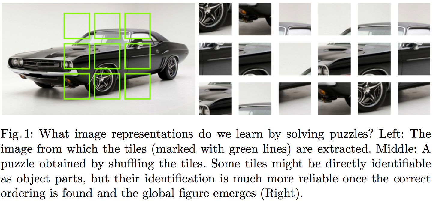
The core idea behind this paper is powerfully simple. The goal is to learn useful representations from unlabelled data, useful in the sense of helping supervised object classification. This paper does this by chopping up images into a set of little jigsaw puzzle, scrambling the pieces, and asking a deep neural network to learn to reassambple them in the correct constellation. A picture is worth a thousand words, so here is Figure 1 taken from the paper explaining this visually:
Summary of this note:
- I note the similarities to denoising autoencoders, which motivate my question: "Can this method equivalently represent the data generating distribution?"
- I consider a toy example with just two jigsaw pieces, and consider using an objective like this to fit a generative model $Q$ to data
- I show how the jigsaw puzzle training procedure corresponds to minimising a difference of KL divergences
- Conclude that the algorithm ignores some aspects of the data generating distribution, and argue that in this case it can be a good thing
What does this learn do?
This idea seems to make a lot of sense. But to me, one interesting question is the following:
What does a network trained to solve jigsaw puzzle learn about the data generating distribution?
Motivating example: denoising autoencoders
At one level, this jigsaw puzzle approach bears similarities to denoising autoencoders (DAEs): both methods are self-supervised: they take an unlabelled data and generate a synthetic supervised learning task. You can also interpret solving jigsaw puzzles as a special case 'undoing corruption' thus fitting a more general definition of autoencoders (Bengio et al, 2014).
DAEs have been shown to be related to score matching (Vincent, 2000), and that they learn to represent gradients of the log-probability-density-function of the data generating distribution (Alain et al, 2012). In this sense, autoencoders equivalently represent a complete probability distribution up to normalisation. This concept is also exploited in Harri Valpola's work on ladder networks (Rasmus et al, 2015)
So I was curious if I can find a similar neat interpretation of what really is going on in this jigsaw puzzle thing. If you equivalently represent all aspects of a probability distribution this way? Are there aspects that this representation ignores? Would it correspond to a consistent denisty estimation/generative modelling method in any sense? Below is my attempt to figure this out.
A toy case with just two jigsaw pieces
To simplify things, let's just consider a simpler jigsaw puzzle problem with just two jigsaw positions instead of 9, and in such a way that there are no gaps between puzzle pieces, so image patches (now on referred to as data $x$) can be partitioned exactly into pieces.
Let's assume our datapoints $x^{(n)}$ are drawn i.i.d. from an unknown distribution $P$, and that $x$ can be partitioned into two chunks $x_1$ and $x_2$ of equivalent dimensionality, such that $x=(x_1,x_2)$ by definition. Let's also define the permuted/scrambled version of a datapoint $x$ as $\hat{x}:=(x_2,x_1)$.
The jigsaw puzzle problem can be formulated in the following way: we draw a datapoint $x$ from $P$. We also independently draw a binary 'label' $y$ from a Bernoulli($\frac{1}{2}$) distribution, i.e. toss a coin. If $y=1$ we set $z=x$ otherwise $z=\hat{x}$.
Our task is to build a predictior, $f$, which receives as input $z$ and infers the value of $y$ (outputs the probability that its value is $1$). In other words, $f$ tries to guess the correct ordering of the chunks that make up the randomly scrambled datapoint $z$, thereby solving the jigsaw puzzle. The accuracy of the predictor is evaluated using the log-loss, a.k.a. binary cross-entropy, as it is common in binary classification problems:
$$
\mathcal{L}(f) = - \frac{1}{2} \mathbb{E}_{x\sim P} \left[\log f(x) + \log (1 - f(\hat{x}))\right]
$$
Let's consider the case when we express the predictor $f$ in terms of a generative model $Q$ of $x$. $Q$ is an approximation to $P$, and has some parameters $\theta$ which we can tweak. For a given $\theta$, the posterior predictive distribution of $y$ takes the following form:
$$
f(z,\theta) := Q(y=1\vert z;\theta) = \frac{Q(z;\theta)}{Q(z;\theta) + Q(\hat{z};\theta)},
$$
where $\hat{z}$ denotes the scrambled/permuted version of $z$. Notice that when $f$ is defined this way the following property holds:
$$
1 - f(\hat{x};\theta) = f(x;\theta),
$$
so we can simplify the expression for the log-loss to finally obtain:
\begin{align}
\mathcal{L}(\theta) &= - \mathbb{E}_{x \sim P} \log Q(x;\theta) + \mathbb{E}_{x \sim P} \log [Q(x;\theta) + Q(\hat{x};\theta)]\\
&= \operatorname{KL}[P|Q_{\theta}] - \operatorname{KL}\left[P\middle|\frac{Q_{\theta}(x)+Q_{\theta}(\hat{x})}{2}\right] + \log(2)
\end{align}
So we already see that using the jigsaw objective to train a generative model reduces to minimising the difference between two KL divergences. It's also possible to reformulate the loss as:
$$
\mathcal{L}(\theta) = \operatorname{KL}[P|Q_{\theta}] - \operatorname{KL}\left[\frac{P(x) + P(\hat{x})}{2}\middle|\frac{Q_{\theta}(x)+Q_{\theta}(\hat{x})}{2}\right] - \operatorname{KL}\left[P\middle|\frac{P(x) + P(\hat{x})}{2}\right] + \log(2)
$$
Let's look at what the different terms do:
- The first term is the usual KL divergence that would correspond to maximum likelihood. So it just tries to make $Q$ as close to $P$ as possible.
- The second term is a bit weird, particularly as comes into the formula with a negative sign. The KL divergence is $0$ if $Q$ and $P$ define the distribution over the set of jigsaw pieces ${x_1,x_2}$. Notice, I used set notation here, so the ordering does not matter. In a way this term tells the loss function: don't bother modelling what the jigsaw pieces are, only model how they fit together.
- The last terms are constant wrt. $\theta$ so we don't need to worry about them.
Not a proper scoring rule (and it's okay)
From the formula above it is clear that the jigsaw training objective wouldn't be a proper scoring rule, as it is not uniquely minimised by $Q=P$ in all cases. Here are two counterexamples where the objective fails to capture all aspects of $P$:
Consider the case when $P=\frac{P(x) + P(\hat{x})}{2}$, that is, when $P$ is completely insensitive to the ordering of jigsaw pieces. As long as $Q$ also has this property $Q = \frac{Q(x) + Q(\hat{x})}{2}$, all KL divergences are $0$ and the jigsaw objective is constant with respect $\theta$. Indeed, it is impossible in this case for any classifier to surpass chance level in the jigsaw problem.
Another simple example to consider is a two-dimensional binary $P$. Here, the jigsaw objective only cares about the value of $Q(0,1)$ relative to $Q(1,0)$, but completely insensitive to $Q(1,1)$ and $Q(0,0)$. In other words, we don't really care how often $0$s and $1$s appear, we just want to know which one is likelier to be on the left or the right side.
This is all fine because we don't use this technique for generative modelling. We want to use it for representation learning, so it's okay to ignore some aspects of $P$.
Representation learning
I think this method seems like a really promising direction for unsupervised representation learning. In my mind representation learning needs either:
- strong prior assumptions about what variables/aspects of data are behaviourally relevant, or relevant to the tasks we want to solve with the representations.
- at least a little data in a semi-supervised setting to inform us about what is relevant and what is not.
Denoising autoencoders (with L2 reconstruction loss) and maximum likelihood training try to represent all aspects of the data generating distribution, down to pixel level. We can encode further priors in these models in various ways, either by constraining the network architecture or via probabilistic priors over latent variables.
The jigsaw method encodes prior assumptions into the training procedure: that the structure of the world (relative position of parts) is more important to get right than the low-level appearance of parts. This is probably a fair assumption.