Notes on iMAML: Meta-Learning with Implicit Gradients

This week I read this cool new paper on meta-learning: it a slightly different approach compared to its predecessors based on some observations about differentiating the optima of regularized optimization.

• Aravind Rajeswaran, Chelsea Finn, Sham Kakade, Sergey Levine (2019) Meta-Learning with Implicit Gradients

Another paper that came out at the same time has discovered similar techniques, so I thought I'd update the post and mention it, although I won't cover it in detail and the post was written primarily about Rajeswaran et al (2019)

• Yutian Chen, Abram L. Friesen, Feryal Behbahani, David Budden, Matthew W. Hoffman, Arnaud Doucet, Nando de Freitas (2019) Modular Meta-Learning with Shrinkage

Outline of this post

• I will give a high-level overview of the meta-learning setup, where our goal is to learn a good initialization or regularization strategy for SGD so it converges to better minima across a range of tasks.
• I illustrate how iMAML works on a 1D toy-example, and discuss the behaviour and properties of the meta-objective.
• I will then discuss a limitation of iMAML: that it only considers the location of minima, and not the probability with which a stochastic algorithm ends up in a specific minimum.
• I will finally relate iMAML to a variational approach to meta-learning.

Meta-Learning and MAML

Meta-learning has several possible formulations, I will try to explain the setup of this paper following my own interpretation and notation that differs from the paper but will make my explanations clearer (hopefully).

In meta-learning we have a series of independent tasks, with associated training and validation loss functions $f_i$ and $g_i$, respectively. We have a set of model parameters $\theta$ which are shared across the tasks, and the loss functions $f_i(\theta)$ and $g_i(\theta)$ evaluate how well the model with parameters $\theta$ does on the training and test cases of task $i$. We have an algorithm that has access to the training loss $f_i$ and some meta-parameters $\theta_0$, and output some optimal or learned parameters $\theta_i^\ast = Alg(f_i, \theta_0)$. The goal of the meta-learning algorithm is to optimize the meta-objective

$$
\mathcal{M}(\theta_0) = \sum_i g_i(Alg(f_i, \theta_0))
$$

with respect to the meta-parameters $\theta_0$.

In early versions of this work, MAML, the algorithm was chosen to be stochastic gradient descent, $f_i$ and $g_i$ being the training and test loss of a neural network, for example. The meta-parameter $\theta_0$ was the point of initialization for the SGD algorithm, shared between all the tasks. Since SGD updates are differentiable, one can compute the gradient of the meta-objective with respect to the initial value $\theta_0$ by simply backpropagating through the SGD steps. This was essentially what MAML did.

However, the effect of initialization on the final value of $\theta$ is pretty weak, and difficult - if at all possible - to characterise analytically. If we allow the SGD to go on for many steps, we might converge to a better parameter, but the trajectory will be very long, and the gradients with respect to the initial value vanish. If we make the trajectories short enough, the gradients w.r.t. $\theta_0$ are informative but we may not reach a very good final value.

iMAML

This is why Rajeswaran et al opted to make the dependence of the final point of the trajectory on meta-paramteter $\theta\_0$ way stronger: Instead of simply initializing SGD from $\theta\_0$ they also anchor the parameter to stay in the vicinity of $\theta\_0$ by adding a quadratic regularizer $\|\theta - \theta_0\|$ to their loss. Because of this, two things happen:

• now all steps of the SGD depend on $\theta$, not just the initial point
• now the location of  the minimum SGD eventually converges to also depend on #\theta\_0#

It is this second property that iMAML exploits. Let me illustrate what that dependence looks like:

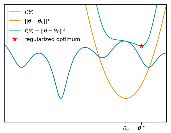
In the figure above, let's say that we would like to minimise an objective function $f(\theta)$. This would be the training loss of one of the tasks the meta-learning algorithm has to solve. Our current meta-parameter $\theta_0$ is marked on the x axis, and the orange curve shows the associated quadratic penalty. The teal curve shows the sum of the objective with the penalty. The red star shows the location of the minimum, which is what the learning algorithm finds.

Now let's animate this plot. I'm going to move the anchor point $\theta_0$ around, and reproduce the same plots. You can see that, as we move $\theta_0$ and the associate penalty, the local (and therefore global) minima of the regularized objective move change:

So it's clear that there is a non-trivial, non-linear relationship between the anchor-point $\theta_0$ and the location of a local minimum $\theta^\ast$. Let's plot this relationship as a function of the anchor point:

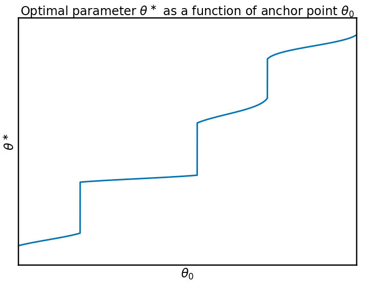
We can see that this function is not at all nice to work with, it has sharp jumps when the closest local minimum to $\theta_0$ changes, and it is relatively flat between these jumps. In fact, you can observe that the sharpest the local minimum nearest to $\theta_0$ is, the flatter the relationship between $\theta_0$ and $\theta$. This is because if $f$ has a sharp local minimum near $\theta_0$, then the location of the regularized minimum will be mostly determined by $f$, and the location of the anchor point $\theta_0$ doesn't matter much. If the local minimum around f is wide, there's a lot of wiggle room for the optimum and the effect of the regularization will be larger.

Implicit Gradients

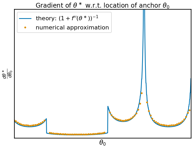
And now we come to the whole point of the iMAML procedure. The gradient of this function $\theta^\ast(\theta_0)$ in fact can be calculated in closed form. It is, indeed, related to the curvature, or second derivative, of $f$ around the minimum we find:

$$
\frac{d\theta^\ast}{d\theta_0} = \frac{1}{1 + f''(\theta^\ast)}
$$

In order to check that this formula works, I calculated the derivative numerically and compared it with what the theory predicts, they match perfectly:

When the parameter space is high-dimensional, we have a similar formula involving the inverse of the Hessian plus the identity. In high dimensions, inverting or even calculating and storing the Hessian is not very practical. One of the main contributions of the iMAML paper is a practical way to approximate gradients, using a conjugate gradient inner optimization loop. For details, please read the paper.

Optimizing the meta-objective

When optimizing the anchor point in a meta-learning setting, it is not the location $\theta^\ast$ we are interested in, only the value that the function $f$ takes at this location. (in reality, we would now use the validation loss, in place of the training loss used for gradient descent, but for simplicity, I assume the two losses overlap). The value of $f$ at its local optimum is plotted below:

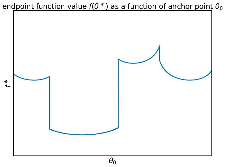
Oh dear. This function is not very pretty. The meta-objective $f(\theta^\ast(\theta_0))$ becomes a piecewise continuous function, a connection of neighbouring basins, with non-smooth boundaries. The local gradients of this function contain very little information about the global structure of the loss function, it only tells you where to go to reach the nearest local minimum. So I wouldn't say this is the nicest function to optimize.

Thankfully, though, this function is not what we have to optimize. In meta-learning, we have a distribution over functions $f$ we optimize, so the actual meta-objective is something like $\sum_i f_i(\theta_i^\ast(\theta_0))$. And the sum of a bunch of ugly functions might well turn into something smooth and nice. In addition, the 1-D function I use for this blog post is not representative of the high-dimensional loss functions of neural networks which we want to apply iMAML to. Take for example the concept of mode connectivity (see e.g. Garipov et al, 2018): it seems that the modes found by SGD using different random seeds are not just isolated basins, but they are connected by smooth valleys along which the training and test error are low. This may in turn make the meta-objective behave more smoothly between minima.

What is missing? Stochasticity

An important aspect that MAML or iMAML do not not consider is the fact that we usually use stochastic optimization algorithms. Rather than deterministically finding a particular local minimum, SGD samples different minima: when run with different random seeds it will find different minima.

A more generous formulation of the meta-objective would allow for stochastic algorithms. If we denote by $\mathcal{Alg}(f_i, \theta_0)$ the distribution over solutions the algorithm finds, the meta-objective would be

$$
\mathcal{M}_{stochastic}(\theta) = \sum_i \mathbb{E}_{\theta \sim \mathcal{Alg}(f_i, \theta_0)} g_i(\theta)
$$

Allowing for stochastic behaviour might actually be a great feature for meta-learning. While the position of the global minimum of the regularized objective can change abruptly s a function $\theta_0$ (as illustrated in the third figure above), allowing for stochastic behaviour might smooth our the meta-learning objective.

Now suppose that SGD anchored to $\theta_0$ converges to one of a finite set of local minima. The meta-learning objective now depends on $\theta_0$ in two different ways:

• as we change the anchor $\theta_0$, the location of the minima change, as illustrated above. This change is differentiable, and we know its derivative.
• as we change the anchor $\theta_0$, the probability with which we find the different solutions changes. Some solutions will be found more often, some less often.

iMAML accounts for the first influence, but it ignores the influence through the second mechanism. This is not to say that iMAML is broken, but that it misses a possibly crucial contribution of stochastic behaviour that MAML or explicitly differentiating through the algorithm does not.

Compare with a Variational Approach

Of course this work reminded me of a Bayesian approach. Whenever someone describes quadratic penalties, all I see are Gaussian distributions.

In a Bayesian interpretation of iMAML, one can think of the anchor point $\theta_0$ as the mean of a prior distribution over the neural network's weights. The inner loop of the algorithm, or $Alg(f_i, \theta_0)$ then finds the maximum-a-posteriori (MAP) approximation to the posterior over $\theta$ given the dataset in question. This is assuming that the loss is a log likelihood of some kind. The question is, how should one update the meta-parameter $\theta_0$?

In the Bayesian world, we would seek to optimize $\theta_0$ by maximising the marginal likelihood. As this is usually intractable, so it is common to turn to a variational approximation, which in this case would look something like this:

$$
\mathcal{M}_{\text{variational}}(\theta_0, Q_i) = \sum_i \left( KL[Q_i\vert \mathcal{N}_{\theta_0}] + \mathbb{E}_{\theta \sim Q_i} f_i(\theta) \right),
$$

where $Q_i$ approximates the posterior over model parameters for task $i$. A specific choice of $Q_i$ is a dirac delta distribution centred at a specific point $Q_i(

theta) = \delta(\theta - \theta^{\ast}_i)$. If we generously ignore some constants that blow up to infinitely large, the KL divergence between the Gaussian prior and the degenerate point-posterior is a simple Euclidean distance, and our variational objective reduces to:

$$
\mathcal{M}_{\text{variational}}(\theta_0, \theta_i) = \sum_i \left( \|\theta_i - \theta_0\|^2 + f_i(\theta_i) \right)
$$

Now this objective function looks very much like the optimization problem that the inner loop of iMAML attempts to solve. If we were working in the pure variational framework, this may be where we leave things, and we could jointly optimize all the $\theta_i$s as well as $\theta_0$. Someone in the know, please comment below pointing me to the best references where this is being done for meta-learning.

This objective is significantly easier to optimize with and involves no inner-loop optimization or black magic. It simply ends up pulling $\theta_0$ closer to the centre of gravity of the various optima found for each task $i$. Not sure if this is such a good idea though for meta-learning, as the final values of $\theta_i$ which we reach by jointly optimizing over everything may not be reachable by doing SGD from $\theta_0$ from scratch. But who knows. A good idea may be, given the observations above, to jointly minimize the variational objective with respect to $\theta_0$ and $\theta_i$, but every once in a while reinitialize $\theta_i$ to be $\theta_0$. But at this point, I'm really just making stuff up...

Anyway, back to iMAML, which does something interesting with this variational objective, and I think it can be understood as a kind of amortized computation: Instead of treating $\theta_i$ as separate auxiliary parameters, it specifies that $\theta_i$ are in fact a deterministic function of $\theta_0$. As the variational objective is a valid upper bound for any value of $\theta_i$, it is also a valid upper bound if we make $\theta_i$ explicitly dependent on $\theta_0$. The variational objective thus becomes a function of $\theta_0$ only (and also of hyperparameters of the algorithm $Alg$ if it has any):

$$
\mathcal{M}_{\text{variational}}(\theta_0) = \sum_i \left( \|Alg(f_i, \theta_0) - \theta_0\|^2 + f_i(Alg(f_i, \theta_0)) \right)
$$

And there we have it. A variational objective for meta-learning $\theta_0$ which is very similar to the MAML/iMAML meta-objective, except it also has the $\|Alg(f_i, \theta_0) - \theta_0\|^2$ term which factors into updating $\theta_0$ which we didn't have before. Also notice that I did not use separate training and validation loss $f_i$ and $g_i$ but that would be a very justified choice as well.

What is cool about this is that this provides extra justification and interpretation for what iMAML is trying to do, and suggests directions in which iMAML could perhaps be improved. On the flipside, the implicit differentiation trick in iMAML might be useful in other situations where we want to amortize the variational posterior similarly.

I'm pretty sure I missed many references, please comment below if you think I should add anything, especially on the variational bit.