Notes on Causally Correct Partial Models
I recently encountered this cool paper in a reading group presentation:
- Rezende et al (2020) Rezende Causally Correct Partial Models for Reinforcement Learning
It's frankly taken me a long time to understand what was going on, and it took me weeks to write this half-decent explanation of it. The first notes I wrote followed the logic of the paper more, this in this post I thought I'd just focus on the high level idea, after which hopefully the paper is more straightforward. I wanted to capture the key idea, without the distractions of RNN hidden states, etc, which I found confusing to think about.
POMDP setup
To start with the basics, this paper deals with the partially observed Markov decision process (POMDP) setup. The diagram below illustrates what's going on:
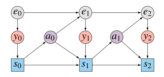
The grey nodes $e_t$ show the unobserved state of the environment at each timestep $t=0,1,2\ldots$. At each timestep the agent observes $y_0$ which depends on the current state of the environment (red-ish nodes). The agent then updates their state $s_t$ based on its past state $s_{t-1}$, the new observation $y_t$, and the previous action taken $a_{t-1}$. This is shown by the blue squares (they're squares, signifying that this node depends deterministically on its parents). Then, based on the agent's state, it chooses an action $a_t$ from by sampling from policy $\pi(a_t\vert s_t)$. The action influences how the environment's state, $e_{t+1}$ changes.
We assume that the agent's ultimate goal is to maximise reward at the last state at time $T$, which we assume is a deterministic function of the observation $r(y_T)$. Think of this reward as the score in an atari game, which is written on the screen whose contents are made available in $y_t$.
The ultimate goal
Let's start by stating what we ultimately would like estimate from the data we have. The assumption is that we sampled the data using some policy $\pi$, but we would like to be able to say how well a different policy $\tilde{\pi}$ would do, in other words, what would be the expected score at time $T$ if instead of $\pi$ we used a different policy $\tilde{\pi}$.
What we are interested in, is a causal/counterfactual query:
$$
\mathbb{E}_{\tau\sim\tilde{p}}[r(y_T)],
$$
where $\tau = [(s_t, y_t, e_t, a_t) : t=0\ldots T]$ denotes a trajectory or rollout up to time $T$, and $\tilde{p}$ denotes the generative process when using policy $\tilde{\pi}$, that is:
$$
\tilde{p}(\tau) = p(e_0)p(y_0\vert e_0) \tilde{\pi}(a_0\vert s_0) p(s_0)\prod_{t=1}^T p(e_t\vert a_{t-1}, e_{t-1}) p(y_t\vert e_t) \tilde{\pi}(a_t\vert s_t) \delta (s_t - g(s_{t-1}, y_t))
$$
I called this a causal or counterfactual query, because we are interested in making predictions under a different distribution $\tilde{p}$ than $p$ which we have observations from. The difference between $\tilde{p}$ and $p$ can be called an intervention, where we replace specific factors in the data generating process with different ones.
There are - at least - two ways one could go about estimating such counterfactual distribution:
- model-free, via importance sampling. This method tries to directly estimate the causal query by calculating a weighted average over the observed data. The weights are given by the ratio between $\tilde{\pi}(a_t\vert s_t)$, the probability by which $\tilde{\pi}$ would choose an action and $\pi(a_t\vert s_t)$, the probability it was chosen by the policy that we used to collect the data. A great paper explaining how this works is (Bottou et al, 2013). Importance sampling as the advantage that we don't have to build any model of the environment, we can directly evaluate the average reward from the samples we have, using only $\pi$ and $\tilde{\pi}$ to calculate the weights. The downside, however, is that importance sampling often incredibly high variance estimate, and is only reliable if $\tilde{\pi}$ and $\pi$ are very close.
- model-based, via causal calculus. If possible, we can use do-calculus to express the causal query in an alternative way, using various conditional distributions estimated from the observed data. This approach has the disadvantage that it requires us build a model from the data first. We then use the conditional distributions learned from the data to approximate the quantity of interest by plugging them into the formula we got from do-calculus. If our models are imperfect, these imperfections/approximation errors can compound when the causal estimand is calculated, potentially leading to large biases and inaccuracies. On the other hand, our models may be accurate enough to extrapolate to situations where importance weighting would be unreliable.
In this paper, we focus on solving the problem with causal calculus. This requires us to build a model of observed data, which we can then use to make causal predictions. The key question this paper asks is
How much of the data do we have to model to be able to make the kinds of causal inferences we would like to make?
Option 1: model (almost) everything
One way we can answer the query above is to model the joint distribution of everything, or mostly everything, that we can observe. For example, we could build a full autoregressive model of observations $y_t$ conditioned on actions $a_t$. In essence this would amount to fitting a model to $p(y_{0:T}\vert a_{0:T})$.
If we had such model, we would theoretically be able to make causal predictions, for reasons I will explain later. However, this option is ruled out in the paper because we assume the observations $y_t$ are very high dimensional, such as images rendered in a computer game. Thus, modelling the joint distribution of the whole observation sequence $y_{1:T}$ accurately is hopeless and would require a lot of data. Therefore, we would like to get away without modelling the whole observation sequence $y_{1:T}$, which brings us to partial models.
Option 2: partial models
Partial models try to avoid modelling the joint distribution of high-dimensional observations $y_{1:T}$ or agent-state sequences $s_{0:T}$, and focus on modelling directly the distribution of $r(y_T)$ - i.e. only the reward component of the last observation, given the action-sequence $a_{0:T}$. This is clearly a lot easier to do, because $r(y_T)$ is assumed to be a low-dimensional aspect of the full observation $y_T$, so all we have to learn is a model of a scalar conditioned on a sequence of actions $q_\theta(r(y_T)\vert a_{0:T})$. We know very well how to fit such models to realistic amounts of data.
However, if we don't include either $y_t$ or $s_t$ in our model, we won't be able to make the counterfactual inferences we wanted to make in the first place. Why? Let's look at he data generating process once more:
We are trying to model the causal impact of actions $a_0$ and $a_1$ on the outcome $y_2$. Let's focus on $a_1$. $y_2$ is clearly statistically dependent on $a_1$. However, this statistical dependence emerges due to completely different effects:
- causal association: $a_1$ influences the state of the environment $e_2$, resulting in an observation $y_2$. Therefore, $a_1$ has an direct causal effect on $y_2$, mediated by $e_2$
- spurious association due to confounding: The unobserved hidden state $e_1$ is a confounder between the action $a_1$ and the observation $y_2$. The state $e_1$ has an indirect causal effect on $a_1$ mediated by the observation $y_1$ and the agent's state $s_1$. Similarly $e_1$ has an indirect effect on $y_2$ mediated by $e_2$.
I illustrated these two sources of statistical association by colour-coding the different paths in the causal graph. The blue path is the confounding path: correlation is induced because both $a_1$ and $y_2$ have $e_1$ as causal ancestor. The red path is the causal path: $a_1$ indirectly influences $y_2$ via the hidden state $e_2$.
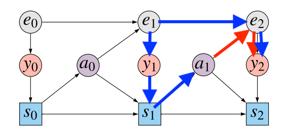
If we would like to correctly evaluate the consequence of changing policies, we have to be able to disambiguate between these two sources of statistical association, get rid of the blue path, and only take the red path into account. Unfortunately, this is not possible in a partial model, where we only model the distribution of $y_2$ conditional on $a_0$ and $a_1$.
If we want to draw causal inferences, we must model the distribution of at least one variable along blue path. Clearly, $y_1$ and $s_1$ are theoretically observable, and are on the confounding path. Adding either of these to our model would allow us to use the backdoor adjustment formula (explained in the paper). However, this would take us back to Option 1, where we have to model the joint distribution of either sequences of observations $y_{0:T}$ or sequences of states $s_{0:T}$, both assumed to be high-dimensional and difficult to model.
Option 3: causally correct partial models
So we finally got to the core of what is proposed in the paper: a kind of halfway-house between modeling everything and modeling too little. We are going to model enough variables to be able to evaluate causal queries, while keeping the dimensionality of the model we have to fit low. To do this, we change the data generating process slightly - by splitting the policy into two stages:
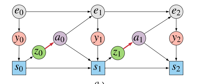
The agent first generates $z_t$ from the state $s_t$, and then uses the sampled $z_t$ value to make a decision $a_t$. One can understand $z_t$ as being a stochastic bottleneck between the agent's high-dimensional state $s_t$, and the low-dimensional action $a_t$. The assumption is that the sequence $z_{0:T}$ should be a lot easier to model than either $y_{0:T}$ or $s_{0:T}$. However, if we now build a model $p(r(y_T), z_{0:T} \vert a_{0:T})$ are now able to use this model evaluate the causal queries of interest, thanks for the backdoor adjustment formula. For how to precisely do this, please refer to the paper.
Intuitively, this approach helps by adding a low-dimensional stochastic node along the confounding path. This allows us to compensate for confounding, without having to build a full generative model of sequences of high-dimensional variables. It allows us to solve the problem we need to solve without having to solve a ridiculously difficult subproblem.