Idea of the Week: Maximum Spacing Estimation, Gaussianisation and Autoregressive Processes
Regular readers of this blog may have realised I am developing an obsession with different objective functions one could use for unsupervised learning. In this post I review objective functions that are based on the idea of Gaussianisation, and then say a few words on how these ideas may be useful for training new types of deep models. Huge thanks to Lucas Theis and Reshad Hosseini whose thesis I recommend for reading. Here's a summary:
- I explain a cute little idea from statistics called maximum spacing estimation, which relies on the observation that squashing a random variable through its cumulative distribution produces a uniform variable.
- I'll then explore how this idea could be used in autoregressive image models, and borrow some pictures from [Reshad Hosseini]'s PhD thesis to illustrate the process called Gaussianisation.
- then, I talk about construct new training objectives for deep generative image models along the lines of adversarial training and kernel moment matching.
- key observation: one can do analytic kernel moment matching or adversarial training in the Gaussianised space, without having to sample! Sampling is one of the killers of adversarial-type methods.
- I think that these objectives can be used to train a deep generative image model composed of alternating layers of autoregressive models, where likelihood-based training would not be possible
Maximum spacing estimation
MSE or maximum spacing estimation relies on the following fact:
$$F(x) = \mathbb{P}(X\leq x) \implies F(X) \sim \mathcal{U}(0,1),$$
That is, if you squash a random variable $X$ through its cumulative distribution function (cdf) $F$, the transformed variable $F(X)$ follows a standard uniform distribution between $0$ and $1$. Furthermore, we can say that for any random variable $X$, its CDF $F$ is the only monotonic, left-continuous function with this property.
Using this observation one can come up with objective functions for univariate density estimation. Let's assume we have a parametric family of distributions described by their CDFs $F_{\theta}$, and we want to find the $\theta$ that best fits our observations $x_1,\ldots,x_N$. If $F_{\theta}$ is close to the true CDF of the data distribution, we would expect $F_\theta(x_i)$ to follow a uniform distribution. Therefore, we only need a way to measure the uniformity of $F_\theta(x_i)$ across samples.
Maximum Spacing Estimation (MSE) uses the geometric mean of spacing between ordered samples as an objective function. This turns out to produce a consistent estimator, in some cases works more sensibly than maximum likelihood, notably to solve the German tank problem. To learn more about this estimator the Wikipedia page is a good place start.
Multivatiate extensions and Gaussianization
The problem with maximum spacing estimation is that it only really makes sense for univariate quantities. There has been some research extending this to multivariate cases in various ways, but I am going to look at how to use similar ideas for training autoregressive models.
Autoregressive processes
You can probably also tell I'm a fan of autoregressive models for unsupervised learning. In an AR model the joint distribution of a multivariate quantity is described in terms of multiplying univariate conditional probability distributions. (the autoregressive term is a bit of a misnomer I think, but that's what people started using to describe the same thing I'm talking about)
We like AR models mainly because calculating the likelihood is typically tractable, unlike models based on something like a Boltzmann distribution or Markov random fields. But now I'm mainly interested in them because for the maximum spacing estimation idea to generalise we can only deal with univariate probability distributions, and AR models conveniently use univariate distributions to construct multivariate models. Mathematically an autoregressive model is one that is explicitly expressed as the product below:
$$q(\mathbf{x};\theta) = \prod_{d=1}^{D} q(x_{d}\vert x_{1:d-1};\theta).$$
Examples of now popular models that work like this are RNNs and LSTMs. AR models are a very natural fit for modelling sequences such as text, they also work well as generative models of images. In image models, one needs to order pixels in the image and thus the model itself will depend on this ordering, which is a bit unnatural. Examples of autoregressive image models include spatial LSTMs, NADE, MADE, MCGSMs. I'm going to mainly talk about modelling images as they are nice to look at, and because I think what I'm describing here may remedy the arbitrariness of ordering pixels.
Uniformization, Gaussianization
Now, if a sequence $\mathbf{x}$ is sampled from a process like above , whose conditional CDFs are denoted by $F_\theta$, then the following still holds:
$$ F_\theta(x_{d+1}\vert x_{1:d}) \sim \mathcal{U}(0,1).$$
In other words, if you take a sequence drawn from an autoregressive process, like an RNN, and then you transform this sequence by squashing each variable through the respective conditional CDFs $F_\theta(\cdot \vert x_{1:d})$, you should end up with a sequence of i.i.d. uniform random numbers, essentially uniform white noise. I will refer to this process as uniformization.
So if you take a model and apply it's implied uniformization operation on real data, the uniformity of the sequence you're left with will tell you how well your model fits data. Therefore, if you minimise some criterion that measures the uniformity of the result of uniformization, you get a generalisation of maximum spacing estimation for autoregressive models.
Clearly, we need a little bit stronger measures of uniformity in the multivariate case. Not only do we want to ensure that the uniformized quantities $F_\theta(x_{d+1}\vert x_{1:d})$ are marginally uniformly distributed, but we also need to ensure that they are independent for different $d$. Consequently, the simple maximum spacings estimator does not cut it anymore as it only measures marginal distributions. But not to worry, measuring i.i.d. uniformity in high dimensions is not a very hard problem, more about this later.
Image modelling example: MCGSM
I wanted to see what happens if you take an AR model that was trained on natural images, and then use that to uniformize natural images. I shared my notes on this with Lucas Theis, who has worked on several AR image models, notable Mixtures of conditional Gaussian scale mixtures (MCGSMs) and spatial LSTMs. He then pointed me to prior work on Gaussianization. In essence, Gaussianization is the same as the uniformization process I explained, but where the image is further transformed by the inverse cdf of a Gaussian, so instead of uniforom white noise, you're supposed to get Gaussian white noise.
It turns out, Lucas and his colleagues have already looked at Gaussianization with MCGSM models. Below are a few Gaussianized images taken from Reshad Hosseini's thesis):
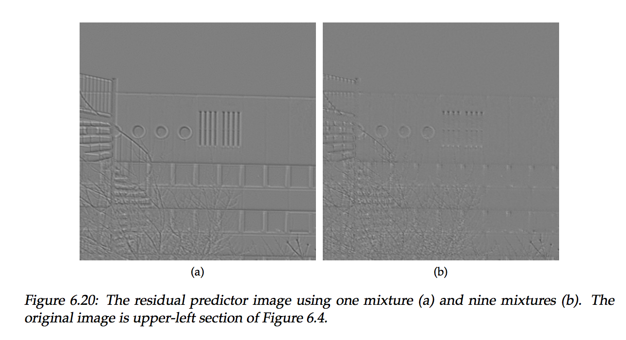
If the generative models were perfect, we would be looking at white Gaussian noise on these images. It's pretty clear that there is still a lot of structure in here, you can pretty much look at this and figure out what the original image was. We can also see that the bigger model produces more i.i.d. looking results, so it seems the bigger model is better at capturing natural image statistics. These models were trained with maximum likelihood, it would be interesting to see what we could get out of these models if we explicitly maximised white-noisiness of these Gaussianised images.
Moment matching in Gaussianized space
Gaussianization opens the way to construct objective functions for unsupervised learning that are based on measures of white-noisiness. For example, one could use an adversarial network or maximum mean discrepancy (MMD) criterion to measure the difference between uniform Gaussian noise and the distribution of Gaussianized images.
The main drawback of both adversarial networks and moment matching networks (MMD) is that to evaluate the training objective one needs to sample from the generative model. Consequently, these methods face a very bad course of dimensionality: you need exponentially more samples to accurately approximate the objective function in high-dimensional spaces. This limits the applicability of these type of techniques to relatively small images, as in LAPGAN.
However, if one applies the MMD criterion in the Gaussianised space, something very useful happens. You are now calculating the MMD between an empirical distribution of Gaussianised images, and a standard normal distribution. Using standard squared-exponential kernels, the integrals in MMD can now be computed in closed form eliminating the need for sampling.
Similar tricks might well work for adversarial training, if the adversarial network uses convolutions and probit activation functions, mean-pooling you can actually analytically calculate the distribution of activations at each layer assuming the input was i.i.d. Gaussian white noise.
Maximum mean discrepancy with Gaussianization provides a closed form objective for training AR image models
Can this be useful in any way?
Now, why might this be useful? It only applies to autoregressive models, and in AR models we can tractably calculate the likelihood anyway, why do we need alternative objective functions? Here is my answer to that: it may give rise to a new class of hierarchical models where likelihood-based training may not work anymore.
The Gaussianised images above hint at a hierarchical approach to density estimation with autoregressive models. As we saw in these images, even if you train a fairly capable model, some structure remains in the Gaussianised image. Now, what if you train another autoregressive model to model the structure that remains in the Gaussianised sequence? Then you squash the Gaussianised data through those CDFs again, and you should get something that is hopefully even closer to standard Normal white noise. Recursively, you can build a hierarchical model botton-up in a greedy fashion layer by layer.
Generating from such a model is relatively straightforward, as long as the conditional CDFs are invertible. You start with uniform white noise on the top layer and transform it with the inverse CDF of each layer in a top-down fashion.
If the stacked autoregressive models are compatible, i.e. they order the pixels in the image in exactly the same way, the likelihood of the resulting hierarchical model could, in fact, be still tractable. So you could even train all layers simultaneously using maximum likelihood.
Stacking AR of different direction
One of the limitations of autoregressive models is that you have to come up with an ordering of pixels in an image. This is a bit arbitrary as there isn't a single natural way to do this. Models such as NADE or MADE get around this limitation by considering ensembles of AR models that work on different permutations of dimensions.
In the hierarchical case, it would be so much more interesting if we could stack AR models that sweep the image using a different ordering of pixels. For example, the bottom layer learns a model over a top-left to bottom-right ordering of pixels, while the layer above it uses an opposite ordering. In this case, you get a generative model whose likelihood is not tractable anymore. The model itself would be a bit like a quasi-Gibbs stochastic generative network. However, it is still straightforward to sample from a model like this, and it is still possible to calculate the Gaussianised images at each layer. Hence, one could use MMD in the Gaussianised space to train these models. I'm not sure how interesting this would be but it's perhaps worth a try.