Invariant Risk Minimization: An Information Theoretic View
I finally got around to reading this new paper by Arjovsky et al. It debuted on Twitter with a big splash, being decribed as 'beautiful' and 'long awaited' 'gem of a paper'. It almost felt like a new superhero movie or Disney remake just came out.
- Martin Arjovsky, Léon Bottou, Ishaan Gulrajani, David Lopez-Paz (2019) Invariant Risk Minimization
The paper is, indeed, very well written, and describes a very elegant idea, a practical algorithm, some theory and lots of discussion around how this is related to various bits. Here, I will describe the main idea and then provide an information theoretic view on the same topic.
Summary of the approach
We would like to learn robust predictors that are based on invariant causal associations between variables, rather than spurious surface correlations that might be present in our data. If we only observe i.i.d. data from a generative process, this is generally not possible.
In this paper, the authors assume that we have access to data sampled from different environments $e$. The data distribution in these different enviroments is different, but there is an underlying causal dependence of the variable of interest $Y$ on some of the observed features $X$ that remains constant, or invariant across all environments. The question is, can we exploit the variability across different environments to learn this underlying invariant association?
Usual empirical risk minimisation (ERM) approaches cannot distinguish between statistical associations that correspond to causal connections, and those that are just spurious correlations. Invariant Risk Minimization can, in certain situations. It does this by finding a representation $\phi$ of features, such that the optimal predictor is simultaneously Bayes optimal in all environments.
The authors then propose a practical loss function that tries to capture his property:
$$
\min_\phi \sum_e \mathcal{R}^e(\Phi) + \lambda \|\nabla_{w\vert w=1}\mathcal{R}^e(w \cdot \Phi)\|^2_2
$$
The first term is the usual ERM: we're trying to minimize average risk across all environments, using a single predictor $\phi$. The second term is where the interesting bit happens. I said before that what we want this term to encorage is that $\phi$ is simultaneously Bayes-optimal in all environments. What the term actually looks at is whether $\phi$ is locally optimal, wether it can be improved locally by scaling by a constant $w$. For details, I recommend reading the paper where a lot of intuitive explanation is provided. In this post, I'll focus on an information theoretic interpretation of what's going on.
Information theoretic explanation
Unlike the authors, who treat the environment index $e$ as something outside of the structural equation model, I prefer to think of $E$ as also being part of the generative process: an observable random variable. This may not be the most useful formulation in all circumstances, but it will help when trying to derive IRM through the lens of conditional dependence relationships.
The most general generative model of data in the IRM setup looks something like this:
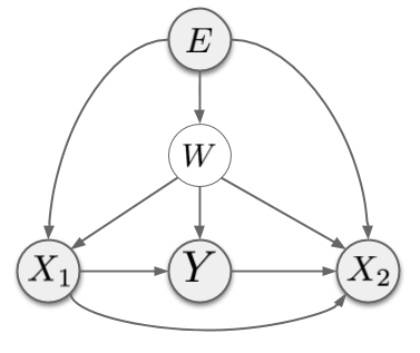
There are three (sets of) observable variables: $E$, the environment index, $X$, the features describing the datapoint and $Y$, the label we wish to predict. I also assume the existence of a hidden confounder $W$. In the above graph, I separated $X$ into upstream dimensions $X_1$ and downstream dimensions $X_2$ based on where they are in the causal chain relative to $Y$. In reality, we don't know what this breakdown is, and breaking $X$ up to $X_1$ and $X_2$ may not be trivial due to entanglement, but it is still reasonable to assume that some components of the input $X$ encode causal parents of $Y$, and others encode causal descendants of $Y$.
The environment $E$ influences every factor in this generative model, except the factor $p(Y\vert X_1, W)$: notice there is no arrow from $E$ to $Y$. In other words, it is assumed that the relationship of variable $Y$ to its observable causal parents $X_1$ and hidden variables $W$ is stable across all environments. This is the primary underlying assumption of IRM. Now, let's read out some conditional independence relationships from this graph:
- $Y \cancel{\perp\mkern-13mu\perp} E$: this is simply saying that the marginal distribution of $Y$ can, generally, change across environments.
- $Y \perp\mkern-13mu\perp E\vert X_1, W$: The observable $X_1$ and latent $W$ shield the label $Y$ from the influence of the environment. I already said that this is the key assumption on which IRM is based: that there is an underlying causal mechanism determining the value of Y from its causal parents, which does not change across environments.
- $Y \cancel{\perp\mkern-13mu\perp} E\vert X_1$: If we leave $W$ out of the conditioning, the above environment-independence no longer holds. This is because the confounder $W$ inroduces spurious association between $X_1$ and $Y$. This spurious correlation is assumed to be environment-dependent.
- $Y \cancel{\perp\mkern-13mu\perp} E\vert X_1, X_2$: this is, perhaps, the most important point. This dependence statement says that the way $Y$ depends on the observable variables $X = (X_1, X_2)$ is environment-dependent. This can be verified by noticing that $X_2$ is a collider between $E$ and $Y$. Conditioning on a collider introduces spurious correlations (for example, explaining away).
In summary, the association between $X$ and $Y$ will be a result of three sources of correlation:
- real causal relationship between some components of $X$ and $Y$.
- spurious association introduced by the unobserved confounder $W$.
- spurious association introduced by conditioning on parts of $X$ which is are causally influenced by $Y$, rather than the other way around.
In a general, if our generative model describes the world accurately, the conditional independence statements we observed tell us that while the real causal association is stable across environments ($Y \perp\mkern-13mu\perp E\vert X_1, W$), the other two are environment-dependent ($Y \cancel{\perp\mkern-13mu\perp} E\vert X_1$ and $Y \cancel{\perp\mkern-13mu\perp} E\vert X_1, X_2$). Thus, we can eliminate the spurious associations by seeking associations that are stable across environments, i.e. independent of $E$.
One can interpret the objective of Invariant Risk Minimisation as seeking a representation of observable variables $\Phi(x)$, such that:
- $Y \perp\mkern-13mu\perp E\vert \phi(X)$, and
- $\phi$ is informative about $y$, i.e. we can predict $y$ accurately from $\phi(x)$
This is a bit similar to the information bottleneck criterion which would seek a stochasstic representation $Z = \phi(X, \nu)$, $\nu$ being some random noise, by solving the following optimization problem:
$$
\max_{\phi} \left\{ I[Y, Z] - \beta I[X, Z] \right\}
$$
We could similarly attempt to find an invariant repesentation $Z = \phi(X)$ by minimizing an objective like:
$$
\max_{\phi} \left\{ I[Y, Z] - \beta I[Y, E \vert Z] \right\}
$$
Notice, that one can write mutual information $\mathbb{I}[Y, E \vert \phi(X)] $ in the following variational interpretation:
$$
I[Y, E \vert \phi(x)] = \max_q \min_r \mathbb{E}_{x,y,e} [\log q(y\vert \phi(x), e) - \log r(y\vert \phi(x))]
$$
With a little bit of math juggling, we can write the above stability objective in the following form:
\begin{align}
\max_{\phi} \left\{ I[Y, \phi(X)] - \beta I[Y, E \vert \phi(X)] \right\} = \max_\phi \max_r \min_q \mathbb{E}_{x,y,e} \left[\log r(y\vert \phi(x)) - \frac{\beta}{1 + \beta}\log q(y\vert \phi(x), e) \right]
\end{align}
This optimization problem is intuitively already very similar to IRM: we would like a representation $\phi$ so we can predict $y$ from it accurately, but we shouldn't be able to build a much better predictor by overfitting to one of the environments. In other words: here, too, we seek a representation so that the Bayes optimal predictor of $y$ is close to Bayes optimal simultanously in all environments.
Sadly, this is a minimax type of problem, so $\phi$ can only be found with a GAN-like iterative algorithm - something we don't really like, but we're kind of getting used to. It would be interesting to see how such algorithm would work, and if you're aware of this being done already, please feel to point me to the relevant references in the comments section.
From information to gradient penalties
I wanted to add sidenote here that I think we can recover something very similar in spirit to (IRMv1). I leave developing the full connection as a homework to you. Let me just illustrate the basic idea here.
Say we have a parametric family of functions $f(y\vert \phi(x); \theta)$ for predicting $y$ from $\phi(x)$. The conditional information can be approximated as follows:
\begin{align}
I[Y, E \vert \phi(x)] &\approx \min_\theta {E}_{x,y} \ell (f(y\vert \phi(x); \theta) - \mathbb{E}_e \min_{\theta_e} \mathbb{E}_{x,y\vert e} \ell (f(y\vert \phi(x); \theta_e)\\
&= \min_\theta \mathbb{E}_e \mathcal{R}^e(f_\theta\circ\phi) - \mathbb{E}_e \min_{\theta_e} \mathcal{R}^e(f_{\theta_e}\circ\phi)
\end{align}
where $\ell$ is the log-loss, if we want to recover Shannon's information. If we assume that $f$ is a universal function approximator, an equality holds. If, instead of globally optimizating $\theta_e$, we only search locally within a trust region around $\theta$, we can create the following (approximate) lower-bound to the information.
\begin{align}
I[Y, E \vert \phi(x)] &\geq \min_\theta {E}_{x,y}\ell f(y\vert \phi(x); \theta) - \mathbb{E}_e \min_{\|d\|^2\leq \epsilon} \mathbb{E}_{x,y\vert e} \ell f(y\vert \phi(x); \theta + d) \\
&= \min_\theta \mathbb{E}_e \left\{ \mathcal{R}^e(f_\theta\circ\phi) - \min_{\|d_e\|\leq \epsilon}\mathcal{R}^e(f_{\theta + d_e}\circ\phi) \right\}
\end{align}
Now, we can approximate the risk $\mathcal{R}^e(f_{\theta + d_e}\circ\phi) $ locally by a first order Taylor approximation around $\theta$, and show that, as $\epsilon \rightarrow 0$, we obtain that:
$$
I[Y, E \vert \phi(x)] \geq \min_\theta \mathbb{E}_e \| \nabla_\theta \mathbb{E}_{x,y\vert e} [\ell f(y\vert \phi(x), \theta)] \|_2= \min_\theta \mathbb{E}_e \| \nabla_\theta \mathcal{R}^e(f_\theta\circ\phi) \|_2
$$
Compare this with the second term in Eqn IRMv1 of the paper. If we now add back in the requirement that we would like to be able to predict $y$ from $\phi(x)$, we get an optimization problem of the following form:
$$
\min_\phi \left\{ \min_\theta \mathbb{E}_e \mathcal{R}^e(f_\theta\circ\phi) + \lambda \min_\theta \mathbb{E}_e \| \nabla_\theta \mathcal{R}^e(f_\theta\circ\phi) \|_2 \right\},
$$
which is almost like the IRM objective. Technically, there are two minimizations over $\theta$ and there's no reason why the two shouldn't be done separately. Note however, that a global minimum of the second term $\mathbb{E}_e \| \nabla_\theta \mathcal{R}^e(f_\theta\circ\phi) \|_2$ is always a local minimum of the first term. This justifies connecting the two minimization problems together:
$$
\min_\phi \min_\theta \left\{ \mathbb{E}_e \mathcal{R}^e(f_\theta\circ\phi) + \lambda \mathbb{E}_e \| \nabla_\theta \mathcal{R}^e(f_\theta\circ\phi) \|_2 \right\},
$$
This is no longer an ugly minimax problem, however, it is still not amazing. It is a lower bound to the original objective which we originally wished to minimize. The lower bound was created when we replaced global minimization over local minimization. Thus, the bound is actually tight if all local minima with respect to $\theta$ of $\mathcal{R}^e(f_\theta\circ\phi)$ are also global minima, e.g. if the loss is convex. In non-convex problems, all bets are off. It may still work, but who knows.
Summary
This is indeed a nice paper, with lots of great insights. Unfortunately, I am not sure how realistic the assumptions are that we can sample from a multitude of different environments, which differ from each other sufficiently so that the invariant causal quantities can be identified.
Other work on invariance
I would like to mention that this is not the first time that invariance and causality have been connected and exploited for domain adaptation. I personally first encountered this idea in a talk by Jonas Peters at the Causality Workshop in 2018. Here is a related paper by him that I wanted to highlight here:
- Peters, Bühlmann, Meinshausen (2016) Causal inference by using invariant prediction: identification and confidence intervals
And here are two more papers which propose a causal treatment of the domain adaptation problem:
- Adarsh Subbaswamy, Peter Schulam, Suchi Saria (2018) Preventing Failures Due to Dataset Shift: Learning Predictive Models That Transport
- Christina Heinze-Deml, Nicolai Meinshausen (2019) Conditional Variance Penalties and Domain Shift Robustness
The second paper, which commenters also pointed out to me, is perhaps the most closely related, but it is based on slightly different assumptions about what is invariant across the domains.
Finally, commenters asked me about domain-adversarial learning, so I wanted to include a pointer here for completeness:
- Yaroslav Ganin, Victor Lempitsky (2014) Unsupervised Domain Adaptation by Backpropagation
On this paper, I agree with Arjovsky et al (2019)'s discussion in the IRM paper: it promotes the wrong invariance property by trying to learn a data representation that is marginally independent of the domain index. See the discussion on this in the comments section below.
Finally, I wanted to point out another slightly looser connection: non-stationarity, or the availability of data from multiple environments has been exploited by (Hyvarinen and Morioka, 2016) exploits this idea for unsupervised feature learning. It turns out, this non-stationarity and the availability of different environments makes otherwise non-identifiable nonlinear ICA models identifable.