ICML Highlight: Contrastive Divergence for Combining Variational Inference and MCMC

Welcome to my ICML 2019 jetlag special - because what else do you do when you wake up earlier than anyone than write a blog post. Here's a paper that was presented yesterday which I really liked.

• Ruiz and Titsias (2019) A Contrastive Divergence for Combining Variational Inference and MCMC

Background: principle of minimal improvement

First, some background on why I found this paper particulartly interesting. When AlphaGo Zero came out, I wrote a post about the principle of minimal improvement: Suppose you have an operator which may be computationally expensive to run, but which that can take a policy and improve it. Using such improvement operator you can define an objective function for policies by measuring the extent to which the operator changes a policy. If your policy is already optimal, the operator can't improve it any further, so the change will be zero. In the case of AlphaGo Zero, the improvement operator is Monte Carlo Tree Search (MCTS). I noted in that post how the same principle may be applicable to approximate inference: expectation propagation and contrastive divergence both can be casted in a similar light.

The paper I'm talking about uses a very similar argument to come up with a contrastive divergence for variational inference, where the improvement operator is MCMC step.

Combining VI with MCMC

The two dominant ways of performing inference in latent variable models are variational inference (including amortized inference, such as in VAE), and Markov Chain Monte Carlo (MCMC). VI approximates the posterior with a paramteric distribution. This can be computationally efficient and practically convenient as VI results in end-to-end differentiable, unbiased estimates of the evidence lower bound (ELBO). As a drawback, the paramteric posterior approximation often can't approximate the posterior perfectly, and an approximation error almost always remains. By contrast, an MCMC approximate posterior can always be improved by running the chains longer, and obtaining more independent samples, but it is more difficult to work with and computationally more demanding than VI.

A lot of great work has been done recently on combining VI with MCMC (see references in Ruiz and Titsias, 2019). Usually, one starts from a crude, parametric variational approximation to the posterior, and then improves it by running a couple steps of MCMC. Crucially, one can view the transition kernel, $\Pi$, of the MCMC as an improvement operator: given any distribution $q$, taking an MCMC steps should take you closer to the posterior. In other words, $\Pi q$ is an improvement over $q$. Taking multiple steps, i.e. $\Pi^t q$, should provide an even greater improvement. Improvement is $0$ only when $\Pi q = q$ which only holds for the true posterior. It is a reasonable criterion therefore to seek a posterior approximation $q_\theta$ such that the improvement in $\Pi^t q_\theta$ over over $q_\theta$ is minimized.

Two ways to measure improvement

There are two ways of quantifying the amount of improvement, or change, that MCMC provides over a parametric posterior $q_\theta$. The first measures how much closer we got to the posterior $p$ by comparing the KL divergences:

$$
\mathcal{L}_1(\theta) = \operatorname{KL}\left[q_\theta\middle\|p\right] - \operatorname{KL}\left[\Pi^tq_\theta\middle\|p\right]
$$

The second one measures the amount of change between $\Pi^tq_\theta$ and $q_\theta$, measured as the KL divergence. This objective function merely tries to identify fixed points of the improvement operator:

$$
\mathcal{L}_2(\theta) = \operatorname{KL}\left[\Pi^tq_\theta\middle\|q_\theta\right]
$$

Either of these objectives would make sense and is justified on its own right, but sadly neither of them can be evaluated or optimized easily in this case. Both require taking expectations over $\Pi^tq_\theta$, as well as evaluating $\log \Pi^tq_\theta$. However, the brilliant insight in this paper is that when you sum them together, the most problematic terms cancel out, leaving you with a tractable objective to minimise.

$$
\mathcal{L}_1(\theta) + \mathcal{L}_2(\theta) = \mathbb{E}_{z\sim \Pi^t q_\theta} f_\theta(z) -  \mathbb{E}_{z\sim q_\theta} f_\theta(z),
$$

where $f_theta(z) = \log p(z,x) - \log q_\theta(z)$, $x$ is the observed, $z$ the hidden variable.

There is one more technical hurdle to overcome, which is to calculate or estimate the derivative of this objective with respect to $\theta$. The authors propose a REINFORCE-like score function gradient estimator in Eqn. (12), which is somewhat worrying as it is known to have very high variance. The authors propose overcoming this using a control variate. For more details, please refer to the paper.

There is further discussion on the behaviour of this objective function in the limit of infinitely long MCMC paths, i.e. $t\rightarrow\infty$. It turns out, the criterion works like the symmetrized KL divergence $KL[q\|p] + KL[p\|q]$. The difference of this objective from the usual conservative mode and seeking VI objective is neatly illustrated in Figure 1 of the paper:

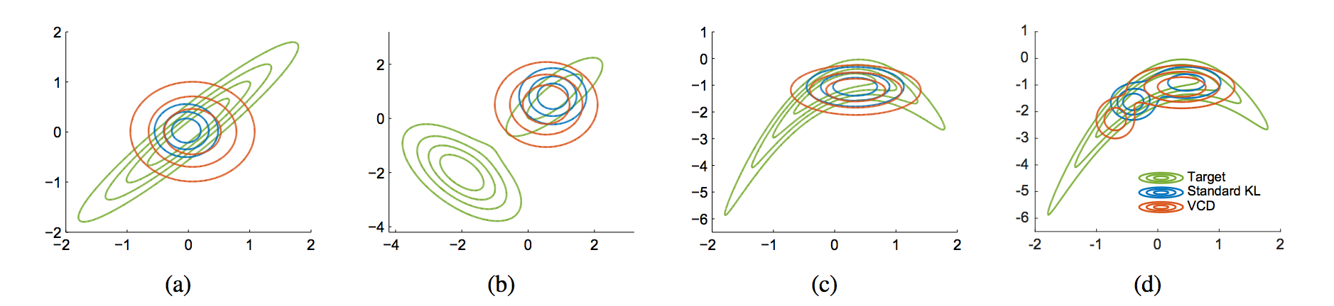
Variational Contrastive Divergence (VCD) favours posterior approximations which have a much higher coverage of the true posterior compared to VI, which tries to cover the modes and tries to avoid allocating mass to areas where the true posterior does not.