
Gaussian Distributions are Soap Bubbles
This post is just a quick note on some of the pitfalls we encounter when dealing with high-dimensional problems, even when working with something as simple as a Gaussian distribution.
Last week I wrote about mixup a new data-augmentation scheme that achieves good performance in a few domains. I illustrated how the method works in a two-dimensional example. While I love understanding problems visually, it can also be problematic, as things work very, very differently in high-dimensions. Even something as simple as a Gaussian distribution does.
Summary of this post:
- in high dimensions, Gaussian distributions are practically indistinguishable from uniform distributions on the unit sphere.
- when drawing figures with additive Gaussian noise, a useful sanity check is normalizing your Gaussian noise samples and see how that changes the conclusions you would draw.
- you should be careful when using the mean or the mode to reason about a distribution in a high-dimensional space (e.g. images). The mode may look nothing like typical samples.
- you should also be careful about linear interpolations in latent spaces where you assume a Gaussian distribution.
Soap bubble
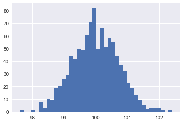
One of the properties of the Gaussian distributions is that in high-dimensions, it is almost indistinguishable from a uniform distribution over a unit-sphere. Try drawing a 10k dimensional standard normal and then calculate the Euclidean norm: It's going to be pretty close to 100, which is square root of dimensions. Here's a histogram of the norm of 1000 different samples from a 10k standard normal:
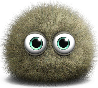
If I show you a Gaussian distribution in 3D and ask you to find a physical metaphor for it, I think at least some of you would reasonably describe it as something like a ball of mold: it's kind of soft or fluffy but gets more and more dense in the middle. Something like this guy:
But in high-dimensional spaces, the image you should have in your mind is more like a soap bubble:
Here's a tool I sometimes use - not nearly often enough - to double check my intuitions: explicitly replace Gaussian distributions with a uniform over the unit ball, or in case of sampling: normalize my Gaussian samples so they all more or less have the same norm. For example, let's see what happens when we look at instance noise or Gaussian data augmentation through this lens:
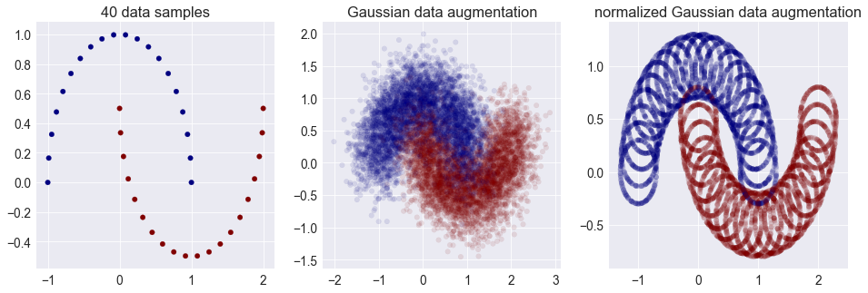
Oops. That doesn't look very nice, does it? So whenever you think about additive Gaussian noise as convolving a distribution with a smooth Gaussian kernel, try to also think about what happens if you convolved your distribution with a circle instead. In high-dimensional spaces the two are virtually indistinguishable from each other.
Mode vs typical samples
Another example of how reasoning can go wrong is looking at the mode of a distribution and expecting it to look like typical random samples drawn from the distribution. Consider image samples where the distribution is drawn from Gaussian distribution:
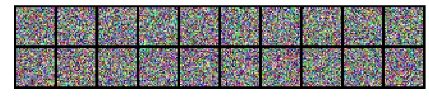
What does the mean or mode of this distribution look like? Well, it's a grey square. It looks nothing like the samples above. What's worse, if instead of white noise, you would consider correlated noise, and then looked at the mode, it could still be the same grey square.
Looking at the mode of the distribution can therefore be misleading. The maximum of a distribution may look nothing like typical samples from a distribution. Consider the beautiful images from the recent feature visualization article on distill. I'm going to steal one of the beautiful pictures here, otherwise please go read and look at the entire thing.
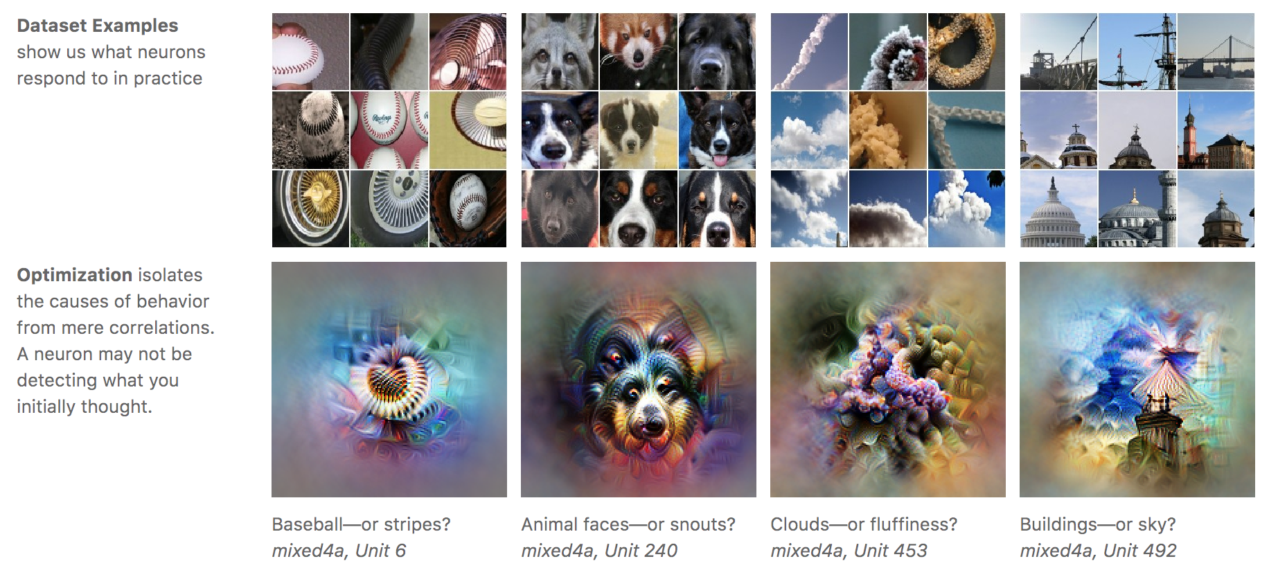
The top panels show images sampled from the training dataset where the neuron's activations are high. The bottom images are obtained by optimizing the input to maximize the response. Therefore one of the bottom images is a little bit like the mode of a distribution, while the corresponding top images are a bit like random samples from the distribution (not quite, but in essence).
The fact that these don't look like each other should not be surprising in itself. If, say, a neuron would respond perfectly to images of Gaussian noise, then the input which maximizes it's activation may look like a grey square, nothing like the samples on which it typically activates and nothing like samples from a Gaussian distribution it has learnt to detect. Therefore, while these images are really cool, and beautiful, their diagnostic value is limited in my opinion. One should not jump to the conclusion that 'the neuron may not be detecting what you initially thought' because the mode of a distribution is not really a good summary in high dimensions.
This is complicated even more by the fact that when we look at an image, we use our own visual system. The visual system learns by being exposed to natural stimuli, which are usually modeled as random samples from a distribution. Our retina has never seen the mode of the natural image distribution, so our visual cortex may not even know how to respond to it, we might find it completely weird. If somebody showed the world the mode of their perfect image density model, we could probably still not tell if it is correct or not because no one has ever seen the original.
Interpolation
UPDATE: Previously this section incomplete: I failed to mention that my interpolation scheme only works if the two endpoints are orthogonal which tends to happen with high probability in high dimensions. Thanks for @Phantrosity for highlighting this.
The last thing I wanted to mention about Gaussians and high dimensional spaces is linear interpolation. If you take two samples, $x_1$ and $x_2$ from a Gaussian distribution in a high-dimensional space, they will both have roughly the same Euclidean norm, and they will be roughly orthogonal. When you consider a convex combination $p x_1 + (1 - p) x_2$ that convex combination has a norm that is proportional to $\sqrt{p^2 + (1 - p)^2} < 1$. Therefore, interpolating this way takes you inside the soap bubble (hence the name convex combination, BTW). If you want to interpolate between two random without leaving the soap bubble you should instead interpolate in in polar coordinates, for example by doing $\sqrt{p} x_1 + \sqrt{(1 - p)} x_2$ as illustrated below:
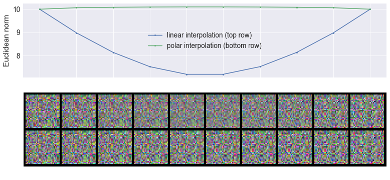
This figure shows the effect of interpolating linearly in cartesian space (top row ) or linearly in polar space (bottom row) between two Gaussian images (left and right). The plot at the top shows how the norm changes as we interpolate linearly or in polar space, you can see that midway between the two images, the norm is quite a bit lower than the norm of either endpoints. You can actually see that linear interpolation results in 'fainter' interpolants.
So generally, when interpolating in latent spaces of something like a VAE or a GAN where you assume the distribution was Gaussian, always interpolate in polar coordinates, rather than in cartesian coordinates. As kindly pointed out by commenters, the scheme I proposed here only works well if the endpoints are independently sampled from a high-D Gaussian and therefore approximately form an orthonormal basis. For a more robust spherical interpolation scheme you might want to opt for something like SLERP.
Inner products
Did I mention two random samples drawn from a standard Normal in a high-dimensional space are orthogonal to each other with a very high probability? Well, they are.