Grosse's challenge: duality and exponential families
I wrote this post in response to a challenge by Roger Grosse:
Theorem 2 of my moment averaging paper is one of the most surprising mathematical results I've seen in machine learning. The proof is very short, but I still have no intuition for why it's true. $500 reward for a clear & convincing intuitive explanation.https://t.co/WjAMg3qIRm
— Roger Grosse (@RogerGrosse) November 27, 2017
As a consequence of responding to a question, this will be a bit of an obscure post, and it may not be very meaningful outside the context of annealed importance sampling. Nevertheless, the post gives me a chance to talk about some interesting aspects of Bregman divergences, exponential families, and hopefully teach some you some new things you may not have come across before.
- Grosse, Maddison and Salakhutdinov (NIPS 2013) Annealing between distributions by averaging moments
If you look further down the thread below Roger's email, it seems @AIActorCritic started answering the question in terms of duality of parametrizations - my post also generalizes things along the lines of duality but goes into a bit more detail.
Summary
- I start with a summary of the results Roger referred to in his tweet.
- Roger found it surprising that Eqns (18) and (19) give the same result.
- I first note that the RHS of Eqns. (18) and (19) is not just something arbitrary, but it is actually the Jeffreys divergence (symmetrized KL) between the endpoints of the path. This gives us hope that there's maybe a more general phenomenon at work here.
- I will then generalize the results by replacing the KL divergence with a more general class of Bregman divergences, and show that the integral of infinitesimal divergences along a linear path will always yield the symmetrized divergence between the endpoints.
- I still lack intuition as to why this actually happens, but I will draw some pretty pictures about Bregman divergences nevertheless.
- then I note the equivalence of Bregman divergences under convex duality, and show that Eqns. (18) and (19) are special cases of the general result for a dual pair of Bregman divergences, both equivalent to the KL divergence. This explains why the two paths give equivalent results.
- Finally, I touch upon how this general Bregman divergence formulation might provide a way to analyze linear interpolation in other parameter spaces.
Introduction
Context: the authors analyze the bias of an Annealed Importance Sampling (AIS) estimator, whose goal is to estimate the normalizing constant of an intractable distribution $p$. AIS constructs a path in the space of probability distributions starting from a tractable distribution $q$ and ending at $p$ via a sequence of intermediate distributions $q=p_0,p_1, \ldots, p_{K-1}, p_K=p$. This path is then used to construct an estimator to the log-partition function (normalizing constant) of $p$. Crucially, the bias of this estimator depends on, among other things, the particular path we take between the two distributions: there are multiple paths between $q$ and $p$, and these paths can result in lower or higher bias. Under some simplifying assumptions the bias is given by:
$$
\delta = \sum_{k=0}^{K-1} D_{KL}[p_k|p_{k+1}].
$$
It is not hard to show that as $K\rightarrow \infty$, this bias vanishes, but what the paper looks at is its precise asymptotic behaviour, with the main insight being Eqn (4):
$$
K\delta \rightarrow \int_0^1 \dot{\theta}(\beta)^\top G_\theta(\beta)\dot{\theta}(\beta) d\beta =:\mathcal{F}(\gamma),
$$
where $\gamma$ denotes the path as a whole, $\theta(\beta), \beta\in[0,1]$ is the path we trace in parameter space $\theta$, and $G_\theta(\beta)$ is the Fisher information matrix with respect to $\theta$ evaluated at $\theta(\beta)$.
Intriguingly, if you calculate $\mathcal{F}(\gamma)$ along two very different paths in distribution space - a straight line in natural parameter space or a straight line in moments space - you get exactly the same value. This is despite the fact that these paths clearly path through very different distributions as illustrated very nicely in Figure 1 of the paper.
So the question is: why are these two paths equivalent in this sense? The answer might lie in convex conjugate duality.
First observation
The first observation we can make is that Eqns. (18) and (19) do not only show that the two paths are equivalent, they also shows that the cost can be expressed in terms of the symetrized KL divergence (sometimes called the Jeffreys divergence) between the endpoints:
$$
\mathcal{F}(\gamma_{MA}) = \mathcal{F}(\gamma_{GA}) = \frac{1}{2}\left( D_{KL}[p_{\beta=0}|p_{\beta=1}] + D_{KL}[p_{\beta=1}|p_{\beta=0}] \right).
$$
To prove this, one can simply use the following formula for the $KL$ divergence between two exponential family distributions with natural parameters $\eta'$ and $\eta$:
$$
D_{KL}[p_{\eta'}|p_{\eta}] = A(\eta') - A(\eta) - s^\top(\eta' - \eta),
$$
where $A(\eta) = \log\mathcal{Z}(\eta)$ is the log-partition function, and $s$ denotes the moments of $p_{\eta}$ just like in the paper. This observation is interesting as we may be looking at special cases of a more general result.
Generalization to Bregman divergences
Any convex functional $H$ over a convex domain induces a Bregman divergence, defined between two points $p$ and $q$ as:
$$
D_H(p|q) = H(p) - H(q) - \langle\nabla H(q), p-q \rangle,
$$
where $\langle\rangle$ denotes inner product. I used this notation rather than vector product to emphasize the fact that $p$ and $q$ might be functions or probability distributions not necessarily just finite dimensional vectors. In what follows I switch back to usual vector notation.
Examples of Bregman divergences include the KL divergence between distributions, the squared Euclidean distance between points in a Euclidean space, the maximum mean discrepancy between probability distributions, and many more. To read more about them, I recommend Mark Reid's great summary.
We can replace the KL divergence in $\delta$ by an arbitrary Bregman divergence, which yields the following generalization of Eqn. (4):
\begin{align}
K \sum_{k=0}^{K-1}D_H(p_k|p_{k+1}) &\rightarrow \frac{1}{2}\int_0^1 \dot{p}(\beta)^\top \nabla^2 H(\beta) \dot{p}(\beta) d\beta\\
&= \frac{1}{2}\int_0^1 \dot{\nabla H}(\beta)^\top \dot{p}(\beta) d\beta,
\end{align}
where $\dot{\nabla H}(\beta)$ is the derivative of $\nabla H(p(\beta))$ with respect to $\beta$, and the second line was obtained by applying the chain rule $\dot{\nabla H}(\beta) = \dot{p}(\beta)\nabla^2 H(\beta)$. $\nabla^2 H(\beta)$ is called the metric tensor and it is a generalization of the Fisher information matrix $G_\theta$ before.
It turns out, if we interpolate in $p$-space linearly, that is, trace a path where $p(\beta) = \beta p_1 + (1 - \beta) p_0$, we can express the above integral analytically in terms of the endpoints of the path $p_0$ and $p_1$:
\begin{align}
\frac{1}{2}\int_0^1 \dot{\nabla H}(\beta)\dot{p}(\beta) d\beta &= \frac{1}{2}\int_0^1 \dot{\nabla H}(\beta)^\top d\beta (p_1 - p_0) \\
&= \frac{1}{2} \left( \nabla H(p_1) - \nabla H(p_0) \right)^\top \left( p_1 - p_0 \right)\\
&= \frac{1}{2}\left( D_H(p_1|p_0) + D_H(p_0|p_1) \right).
\end{align}
This final expression is the symmetrized Bregman divergence between the endpoints of the path $p_1$ and $p_0$, a generalization of the symmetrised KL that we found before.
Before showing how this general result is useful to explain the equivalence of Eqns. (18) and (19), I want to take some time to draw some pretty pictures visualizing Bregman divergences, the quantities we are dealing with are.
A bit of graphical intuition
Below is a graphical illustration of a Bregman divergence between two points $p$ and $q$ with respect to some convex potential $H$.
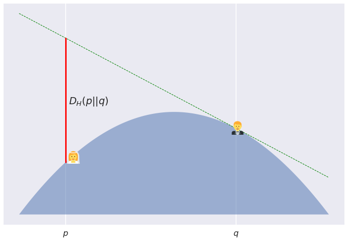
Here's the story: Poppy and Quentin are about to get married. It is bad luck to see each other all dressed up before the wedding. Therefore, they decide to spend the morning on a convex hill (convex from the top). Poppy is at coordinates $p$ and Quentin at $q\neq p$ . The surface of the hill is described by $-H$ where $H$ is a convex function. Precisely because the hill is convex, Quentin can't see Poppy, not unless she starts jumping. The Bregman divergence describes the safe height Poppy is allowed to jump up without Quentin seeing her. The more hilly the hill - higher the curvature - between them, the higher Poppy can jump without being seen by Quentin.
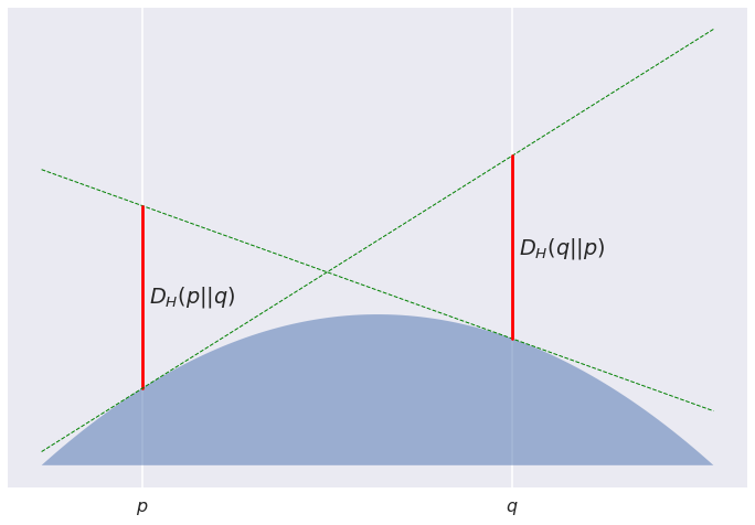
For this figure I used a boring parabolic hill, $-H(p) = p(1-p)$. The resulting divergence actually ends up symmetric and is simply proportional to the squared Euclidean distance $(p-q)^2$:
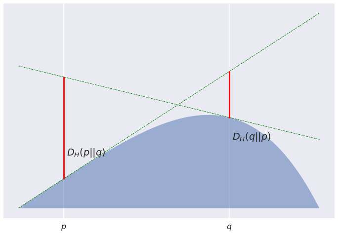
But this is an exception, rather than the rule: most Bregman divergences are asymmetric. For the convex function $H(p) = p(1-p^3)$, this is what the picture looks like:
OK, so what did we just prove before? Consider we have a sequence of bridesmaids equally placed between Poppy and Quentin... Actually, let's stop the wedding analogy before it's too far.
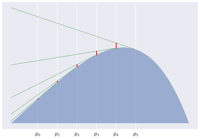
Consider a sequence of points $p_0,\ldots,p_K$ equally placed between $p=p_0$ and $q=p_K$. Now look at the sum of divergences between subsequent points $\sum_k D[p_k,p_{k+1}]$. The divergences say how high each of the $p_k$ has to jump to see $p_{k+1}$. For $K=3$ we are interested in the sum of the red line segments
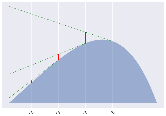
For $K=5$:
For $K=12$:
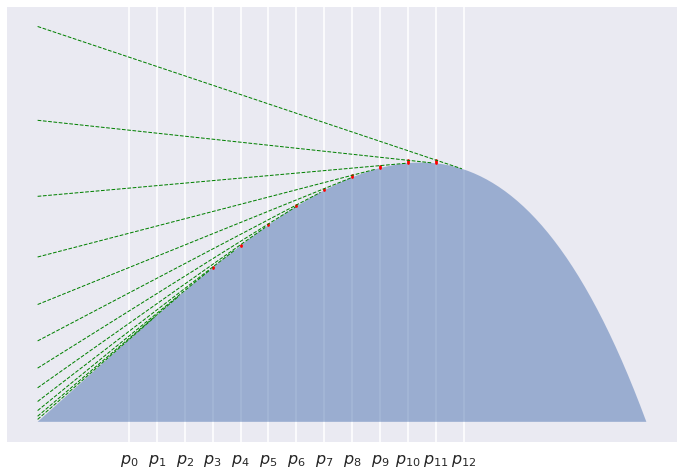
It is pretty clear that the line segments get shorter and shorter, and indeed their sum converges to $0$. What we have proved is that asymptotically this sum behaves like $\frac{1}{2K}\left(D[p|q] + D[q|p]\right)$. Why this is the case is still a mistery to me, and I don't know how to even visualise this. But I wouldn't be surprised if there turned out to be a good reason for this.
Dual Bregman divergences
After a bit an excursion into visualising Bregman divergences in one dimension, let's go back to the question of why linear interpolation in natural parameter-space or moment space gives the $\mathcal{F}(\gamma)$. The answer lies in duality.
Any convex function $H$ defines a Bregman divergence on a convex domain. Any convex function $H$ also has a convex conjugate $H^\ast$. This convex conjugate, $H^\ast$, also defines a Bregman divergence on its own domain, which is generally different from the domain of $H$. Furthermore, this dual divergence is equivalent to the original in the following sense:
$$
D_{H^{\ast}}[p^{\ast}|q^{\ast}] = D_{H}[p|q],
$$
where $p^{\ast} = \nabla H(p)$ and $q_{ast} = \nabla H(q)$ are called the dual parameters corresponding to $p$ and $q$, respectively. The mapping between parameters and dual parameters is one-to-one, thanks to convexity. $p$ and $q$ are sometimes called the primal parameters, but this distinction is rather arbitrary as conjugate duality is a symmetric relationship.
With an understanding of duality, let's look at the formula that we obtained before:
\begin{align}
K \sum_{k=0}^{K-1}D_H(p_k|p_{k+1}) &\rightarrow \frac{1}{2}\int_0^1 \dot{\nabla H}(\beta)^\top \dot{p}(\beta) d\beta,
\\
&= \frac{1}{2}\int_0^1 \dot{p^\ast}(\beta)^\top \dot{p}(\beta) d\beta\\
&= \frac{1}{2}\left(p^\ast(1) - p^\ast(0)\right)^\top\left(p(1) - p(0)\right),
\end{align}
observe the bilinearity of the formula with respect to the primal and dual parameters.
Conjugate duality in exponential families
Let's now consider an exponential family of the form:
$$
p(x\vert \eta) = h(x)\exp(\eta^\top g(x) - A(\eta))
$$
where $A(\eta)=\log\mathcal{Z}(\eta)$ is the log partition function. As $A$ is a convex function of $\eta$, we can define a Bregman divergence in the coordinate system of natural parameters $\eta$ induced by the (convex) log-partition function $A$:
$$
D_A[\eta'|\eta] = A(\eta') - A(\eta) - \nabla A(\eta)^T\left( \eta' - \eta\right).
$$
(notice how similar this is to the KL divergence expression I used before)
The dual parameter corresponding to $\eta$ turns out to be the moments parameters $s$:
$$
\eta^\ast = \nabla A (\eta) = \mathbb{E}_\eta[g(x)] = s,
$$
The equality in the middle is a well-known property of exponential families, the proof is similar to how you would obtain the REINFORCE gradient estimator, for example. Using this equality we can rewrite the divergence above as:
$$
D_A[\eta'|\eta] = A(\eta') - A(\eta) - s^T\left( \eta' - \eta\right).
$$
If we consider the natural parameters $\eta$ the primal parameters, the moments $s$ are the dual parameters. As always, there is a one-to-one mapping between primal and dual parameters. Using the convex conjugate $A^{\ast}$, we can therefore define another Bregman divergence in the coordinate system of moments $s$ as follows:
\begin{align}
D_{A^\ast}[s'|s] &= A^\ast(s') - A^\ast(s) - \nabla A^\ast(s)^T\left(s' - s\right)\\
&= A^\ast(s') - A^\ast(s) - \eta^T\left(s' - s\right)
\end{align}
As it turns out this convex conjugate $A^\ast$ is the negative Shannon's entropy of the distribution parametrized by its moments $s$ (it's beyond this post to show this, see e.g. this book chapter.
So now we have two Bregman divergences, one in the primal space of $\eta$ and one in the dual space $s$. These two divergences are equivalent, and in this case they are also both equivalent to the Kulback-Leibler divergence between the corresponding distributions:
$$
D_{A}[\eta'|\eta] = D_{A^\ast}[s'|s] = D_{KL}[p'|p]
$$
So, putting these things together, we can now understand why Eqns. (18) and (19) give the same result. If we interpolate linearly in primal space between $\eta(0)$ and $\eta(1)$ we get that the loss of the path is:
$$
\mathcal{F}(\gamma_{GA}) = \frac{1}{2}\left( D_A[\eta(1)|\eta(0)] + D_A[\eta(0)|\eta(1)]\right)
$$
Similarly, interpolating between $s(0)$ and $s(1)$ in moment space we obtain:
$$
\mathcal{F}(\gamma_{MA}) = \frac{1}{2}\left( D_{A^\ast}[s(1)|s(0)] + D_{A^\ast}[s(0)|s(1)]\right).
$$
And by the duality of the $A$ and $A^\ast$ we get that the two are equal, and also equal to the symetrized KL divergence between the distributions.
Interestingly, this equivalence also suggests that linear interpolation in the distribution space, $p(\beta) = \beta p_1 + (1 - \beta) p_0$, would also give the same result. This would interpolate between $p_0$ and $p_1$ via mixtures between the two distributions. This option may not be of practical relevance though.
Interpolation in other parameter-spaces
This framework might allow us to study linear interpolation in parameter spaces which are related to natural parameters by a convex operation. So long as $f$ is invertible and $f^{-1}$ has a positive definite Jacobian, we can define a Bregman divergence in $\theta$-space using the convex function $f^{-1}\circ A$. I'm not sure if this would actually work out or whether this would yield any insights.
Summary
This was my attempt at providing more insight into Theorem 2 of Roger's paper he found very surprising. My post probably does little to make the result look less surprising, it merely shifts the surprise elsewhere. The story goes as follows:
- integrating the Bregman divergence along a linear path we obtain the symmetrized Bregman divergence between the endpoints of the path
- For exponential families the KL divergence can be equivalently expressed as a Bregman divergence in natural parameter space or as a Bregman divergence in moments space. The scalar potentials of these divergences are conjugate duals of each other, hence their equivalence.
- Therefore integrating KL divergence along a linear path in either $\eta$ or $s$ space yields the same result, due to the equivalence of the dual Bregman divergences.