My notes on (Liang et al., 2017): Generalization and the Fisher-Rao norm

After last week's post on the generalization mystery, people have pointed me to recent work connecting the Fisher-Rao norm to generalization (thanks!):

• Tengyuan Liang, Tomaso Poggio, Alexander Rakhlin, James Stokes (2017) Fisher-Rao Metric, Geometry, and Complexity of Neural
  Networks

This short presentation on generalization by the coauthors Sasha Rakhlin is also worth looking at - though I have to confess much of the references to learning theory are lost on mesho.

While I can't claim to have understood all the bounding and proofs going on in Section 4, I think I got the big picture so I will try and summarize the main points in the section below. In addition, I wanted to add some figures I did which helped me understand the restricted model class the authors worked with and to understand the "gradient structure" this restriction gives rise to. Feel free to point out if anything I say here is wrong or incomplete.

Norm-based capacity control

The main mantra of this paper is along the lines of results by Bartlett (1998) who observed that in neural networks, generalization is about the size of the weights, not the number of weights. This theory underlies the use of techniques such as weight decay and even early stopping, since both can be seen as ways to keep the neural network's weight vector small. Reasoning about a neural network's generalization ability in terms of the size, or norm, of its weight vector is called norm-based capacity control.

The main contribution of Liang et al (2017) is proposing the Fisher-Rao norm as a measure of how big the networks' weights are, and hence as an indicator of a trained network's generalization ability. It is defined as follows:

$$
|\theta|_{fr} = \theta^\top I_\theta \theta
$$

where $I$ is the Fisher information matrix:

$$
I(\theta) = \mathbb{E}_{x,y} \left[ \nabla_\theta \ell(f_\theta(x),y) \nabla_\theta \ell(f_\theta(x),y)^\top \right]
$$

There are various versions of the Fisher information matrix, and therefore of the Fisher-Rao norm, depending on which distribution the expectation is taken under. The empirical form samples both $x$ and $y$ from the empirical data distribution. The model form samples $x$ from the data, but assumes that the loss is a log-loss of a probabilistic model, and we sample $y$ from this model.

Importantly, the Fisher-Rao norm is something which depends on the data distribution (at least the distribution of $x$). It is also invariant under reparametrization, which means that if there are two parameters $\theta_1$ and $\theta_2$ which implement the same function, their FR-norm is the same. Finally, it is a measure related to flatness inasmuch as the Fisher-information matrix approximates the Hessian at a minimum of the loss under certain conditions.

Summary of the paper's main points:

• in rectified linear networks without bias, the Fisher-Rao norm has an equivalent form which is easier to calculate and analyze (more on this below)
• various other norms previously proposed to bound model complexity can be bounded by the Fisher-Rao norm
• for linear networks without rectification (which in fact is just a linear function) the Rademacher complexity can be bounded by the FR-norm and the bound does not depend on the number of layers or number of units per layer. This suggests that the Fisher-Rao norm may be a good, modelsize-independent proxy measure of generalization.
• the authors do not prove bounds for more general classes of models, but provide intuitive arguments based on its relationship to other norms.
• the authors also did a bunch of experiments to show how the FR-norm correlates with generalization performance. They looked at both vanilla SGD and 2-nd order stochastic method K-FAC. They looked at what happens if we mix in random labels to training, and found that the FR-norm of the final solution seems to track the generalization gap.
• There are still open questions, for example explaining what, specifically, makes SGD converge to better minima, and how this changes with increasing batchsize.

Rectified neural networks without bias

The one thing I wanted to add to this paper, is a little bit more detail on the particular model class - rectified linear networks without bias - that the authors studied here. This restriction turns out to guarantee some very interesting properties, without hurting the empirical performance of the networks (so the authors claim and to some degree demonstrate).

Let's first visualize what the output of a rectified multilayer perceptron with biases looks like. Here I used 3 hidden layers with 15 ReLUs in each and PyTorch-default random initialization. The network's input is 2D, and the output is 1D so I can easily plot contour surfaces:

Figure 1: rectified network with biases

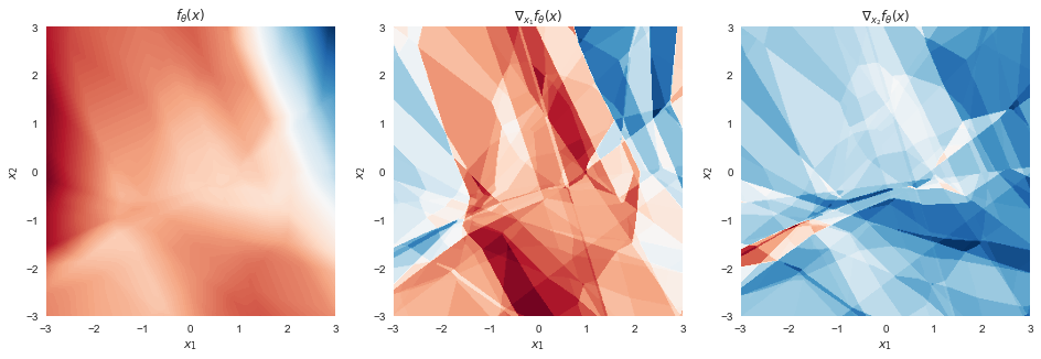
The left-hand panel shows the function itself. The panels next to it show the gradients with respect to $x_1$ and $x_2$ respectively. The function is piecewise linear (which is hard to see because there are many, many linear pieces), which means that the gradients are piecewise constant (which is more visually apparent).

The piecewise linear structure of $f$ becomes more apparent we superimpose the contour plot of the graidents (black) on top of the contour plot of $f$ itself (red-blue):

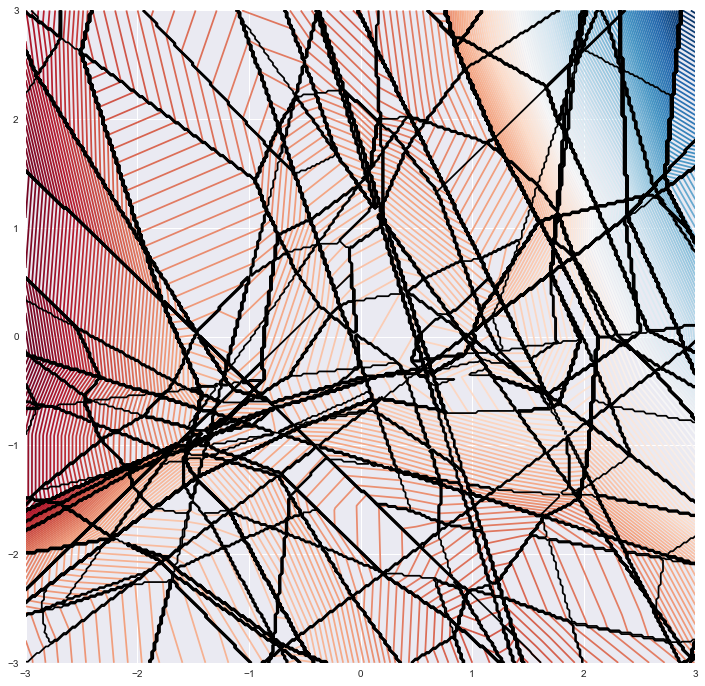
These functions are clearly very flexible and by adding more layers, the number of linear pieces grows exponentially.

Importantly, the above plot would look very similar had I plotted the function's output as a function of two components of $\theta$, keeping $x$ fixed. This is significantly more difficult to plot though, so I'm hoping you'll just believe me.

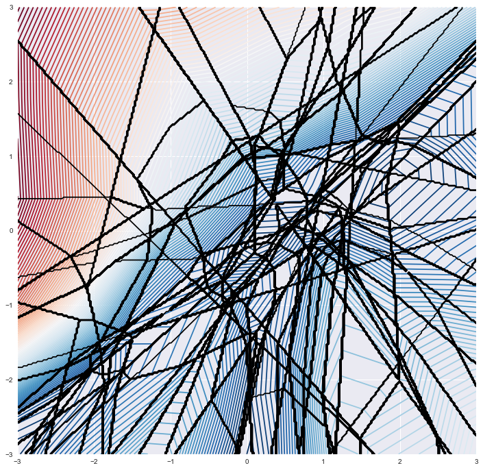
Now let's look at what happens when we remove all biases from the network, keeping only the weight matrices:

Figure 2: rectified network without biases

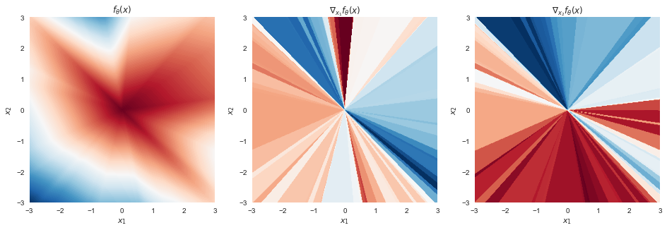
Wow, the function looks very different now, doesn't it? At $x=0$ it always takes the value $0$. It is composed of wedge-shaped (or in higher dimensions, generalized pyramid-shaped) regions within which the functino is linear but the slope in each wedge is different. Yet the surface is still continuous. Let's do the superimposed plot again:

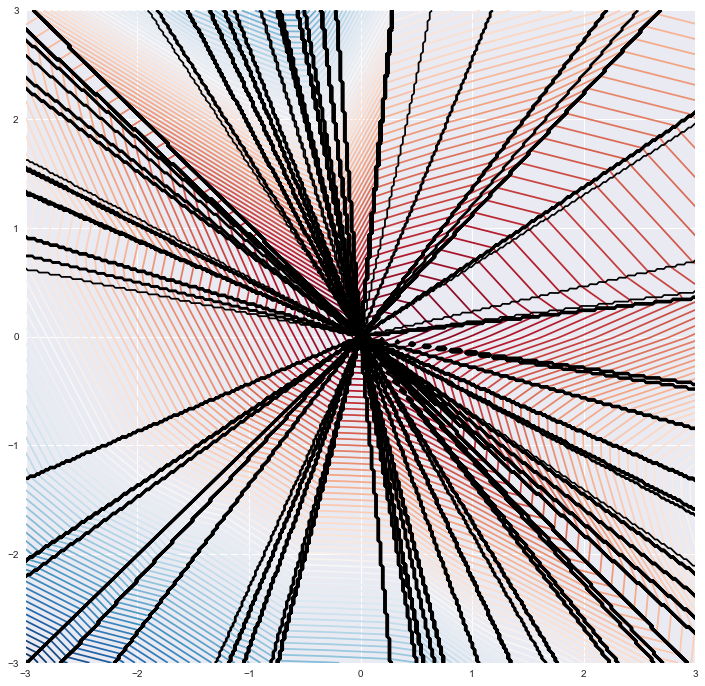
It's less clear from these plots why a function like this can model data just as well as the more general piece-wise linear one we get if we enable biases. One thing that helps is dimensionality: in high dimensions, the probability that two randomly sampled datapoints fall into a the same "pyramind", i.e. share the same linear region, is extremely small. Unless your data has some structure that makes this likely to happen for many datapoints at once, you don't really have to worry about it, I guess.

Furthermore, if my network had three input dimensions, but I only use two dimensions $x_1$ and $x_2$ to encode data and fix the third coordinate $x_3=1$, I can implement the same kind of functions over my inputs. This is called using homogeneous coordinates, and a bias-less network with homogeneous coordinates can be nearly as powerful as one with biases in terms of the functions it can model. Below is an example of a function a rectified network with no biases can implement when using homogeneous coordinates.

Figure 3: rectified network without biases, homogeneous coordinates

This is because the third variable $x_3=1$ multiplied by its weights practically becomes a bias for the first hidden layer.

Second observation is that we can consider $f_\theta(x)$ as a function of the weight matrix of a particular layer, keeping all other weights and the input the same, the function behaves exactly the same way as it behaves with respect to the input $x$. The same radial pattern would be observed in $f$ if I plotted it as a function of a weight matrix (though weight matrices are rarely 2-D so I can't really plot that).

Structure in gradients

The authors note that these functions satisfy the following formula:
$$
f_\theta(x) = \nabla_x f_\theta(x)^\top x
$$

(Moreover I think these are the only continuous functions for which the above equality holds, but I leave this to keen readers to prove or disprove)

Noting the symmetry between the network's inputs and weight matrices, a similar equality can be established with respect to parameters $\theta$:

$$
f_\theta(x) = \frac{1}{L+1}\nabla_\theta f_\theta(x)^\top \theta,
$$

where $L$ is the number of layers.

Why would this be the case?

Here's my explanation which differs slightly from the simple proof the authors give. A general rectified network is piecewise linear with respect to $x$, as discussed. The boundaries of the linear pieces, and the slope, changes as we change $\theta$. Let's fix $\theta$. Now, so long as $x$ and some $x_0$ fall within the same linear region, the function at $x$ equals its Taylor expansion around $x_0$:

\begin{align}
f_\theta(x) &= \nabla_{x} f_\theta(x_0)^\top (x- x_0) + f_{\theta}(x_0) \\
&= \nabla_x f_\theta(x)^\top (x - x_0) + f_{\theta}(x_0)
\end{align}

Now, if we have no biases, all the linear segments are always wedge-shaped, and they all meet at the origin $x=0$. So, we can consider the limit of the above Taylor series in the limit as $x_0\rightarrow 0$. (we have to take a limit only technically as the function is non-differentiable at exactly $x=0$). As $f_{\theta}(0)=0$ we find that

$$
f_\theta(x) = \nabla_x f_\theta(x)^\top x,
$$

just as we wanted. Now, treating layer $l$'s weights $\theta^{(l)}$ as if they were the input to the network consisting of the subsequent layers, and the previous layer's activations as if they were the weight multiplying these inputs, we can derive a similar formula in terms of $\theta^{(l)}$:

$$
f_\theta(x) = \nabla_{\theta^{(l)}} f_\theta(x)^\top \theta^{(l)},
$$

Applying this formula for all layers $l=1\ldots L+1$, and taking the average we obtain:

$$
f_\theta(x) = \frac{1}{L+1}\nabla_\theta f_\theta(x)^\top \theta
$$

We got the $L+1$ from the $L$ hidden layers plus the output layer.

Expression for Fisher-Rao norm

Using the formula above, and the chain rule, we can simplify the expression for the Fisher-Rao norm as follows:

\begin{align}
|\theta|_{fr} &= \mathbb{E} \theta^\top \nabla_\theta \ell(f_\theta(x),y) \nabla_\theta \ell(f_\theta(x),y)^\top \theta \\
&= \mathbb{E} \left( \theta^\top \nabla_\theta \ell(f_\theta(x),y) \right)^2 \\
&= \mathbb{E} \left( \theta^\top \nabla_\theta f_\theta(x) \nabla_f \ell(f,y) \right)^2\\
&= \mathbb{E} \left( f_\theta(x)^\top \nabla_f \ell(f,y)\right)^2
\end{align}

It can be seen very clearly in this form that the Fisher-Rao norm only depends on the output of the function $f_\theta(x)$ and properties of the loss function. This means that if two parameters $\theta_1$ and $\theta_2$ implement the same input-output function $f$, their F-R norm will be the same.

Summary

I think this paper presented a very interesting insight into the geometry of rectified linear neural networks, and highlighted some interesting connections between information geometry and norm-based generalization arguments.

What I think is still missing is the kind of insight which would explain why SGD finds solutions with low F-R norm, or how the F-R norm of a solution is effected by the batchsize of SGD, if at all it is. The other thing missing is whether the F-R norm can be an effective regularizer. It seems that for this particular class of networks which don't have any bias parameters, the model F-R norm could be calculated relatively cheaply and added to as a regularizer since we already calculate the forward-pass of the network anyway.