Exponentially Growing Learning Rate? Implications of Scale Invariance induced by Batch Normalization
Yesterday I read this intriguing paper about the midboggling fact that it is possible to use exponentially growing learning rate schedule when training neural networks with batch normalization:
- Zhiyuan Li and Sanjeev Arora (2019) An Exponential Learning Rate Schedule for Deep Learning
The paper provides both theoretical insights as well as empirical demonstration of this remarcable property.
Scale invariance
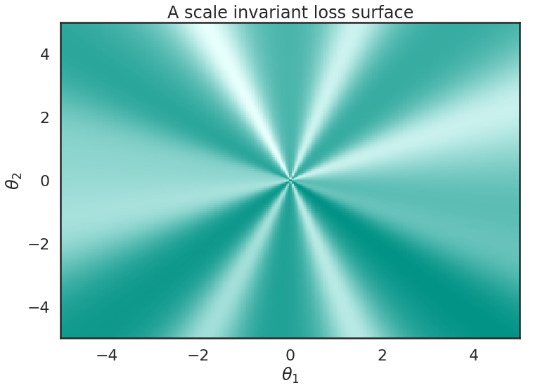
The reason why this works boils down to the observation that batch-normalization renders the loss function of neural networks scale invariant - scaling the weights by a constant does not change the output, or the loss, of the batch normalized network. It turns out that this property alone might result in somewhat unexpected and potentially helpful properties for optimization. I will use this post to illustrate some of the properties of scale invariant loss functions - and gradient descent trajectories on them - using a 2D toy example:

Here, I drew a loss function whih has the scale invariance property. The value of the loss only depends on the angle, but not the magnitude of the weight vector. The value of the loss along any radial line from the origin outwards is constant. Simple consequences of scale invariance are that (Lemma 1 of the paper)
- that the gradient of this function is always orthogonal to the current value of the parameter vector, and that
- the farther you are from the origin, the smaller the magnitude of the gradient. This is perhaps less intuitive but think about how the function behaves on a circle around the origin. The function is the same, but as you increase the radius you stretch the same function round a larger circle - it gets fatter, therefore its gradients decrease.
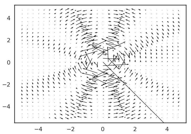
Here is a - somewhat messy - quiver plot showing the gradients of the function above:

The quiver plot is messy because the gradients around the origin explode. But you can perhaps see how the gradients get larger and larger - and remain perpendicular to the value itself.
So Imagine doing vanilla gradient descent (no momentum, weight decay, fixed learning rate) on such a loss surface. Because the gradient is always perpendicular to the current value of the parameter, by the Pythagorean theorem, the norm of the parameter vector increases with each iteration. So gradient descent takes you away from the origin. However, the weight vector won't completely blow up to infinity, because the gradients also get smaller and smaller as the weight vector grows, so it settles at some point. Here is a gradient descent path looks like starting from the coordinate $(-0.7, 0.7)$:

In fact, you can't really see it but the optimization kind of gets stuck in there, and doesn't move any longer. It's interesting to see what happens if we add weight decay, which is the same as adding L2 regularizer over the weights:

We can see that once the trajectory is about to get stuck in a local minimum, weight decay pulls it back towards the origin, which is where gradients become larger. This, in turn, perturbs the trajectory often pushing it out of the current local minimum. So in a way, we can start to build the intuition that weight decay on a scale-invariant loss function acts as a kind of learning rate adjustment.
In fact, what the paper works out is an equivalence between two things:
- weight decay with constant learning rate and
- no weight decay and an exponentially growing learning rate
On the plot below I show the trajectory with the exponentially growing learning rate which is equivalent to the one I showed before with weight decay. This one has no weight decay, and its learning rate keeps growing:

We can see that the trajectory blows up, and quickly gets out of bound on this animation. How can this be equivalent to the weight decay trajectory? Well, from the perspective of the loss function, the magnitude of the weight vector is irrelevant, and we only care about the angle when viewed from the origin. Turns out, if you look at those angles, the two trajectories are the same. To illustrate this, I use the normalization formula from Theorem 2.1 to project this trajectory back to the same magnitude the weight decay one would have. I obtain something that indeed looks very much like the trajectory above:

After a while, the trajectories start working differently, which I think is probably due to the accumulation of numerical errors in my implementation of the toy example. I could probably fix this, but I'm not sure it's worth the effort. The authors show much more convincing empirical evidence that this works in real, complicated neural network losses that people actually want to optimize.
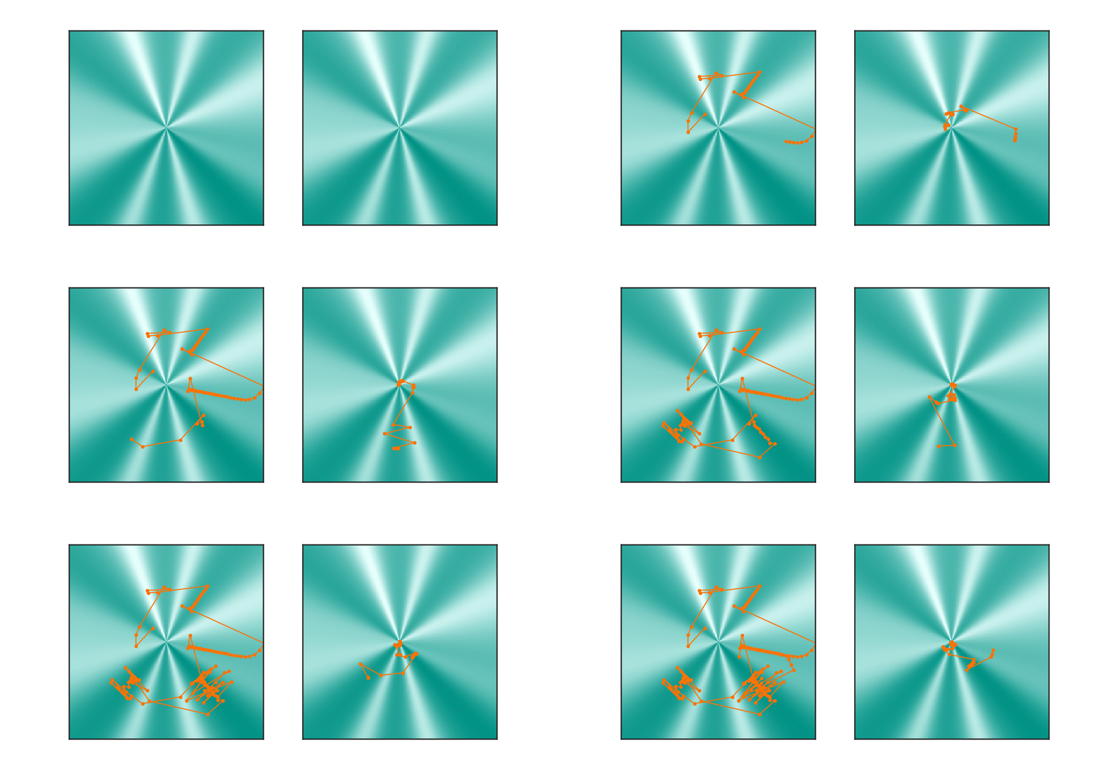
You can think of this renormalization I did above as "constantly zooming out" on the loss landscape to keep up with the exponentially exploding parameter. I tried to illustrate this below:

On the left-hand plot, I show the original, weight-decayed gradient descent with a constant learning rate. On the right-hand plot I show the equivalent trajectory with exponentially growing learning rate and no weight decay, and I also added a constant zoom to counteract the explosion of the parameter's norm, in line with Theorem 2.1. We can see that, especially initially, the two paths behave the same way when viewed from the origin. They then work differently which I believe is down to the numerical precision issue that could probably be worked out.
The paper shows a similar equivalence in the presence of momentum as well, if interested, read the details in the paper.
Summary
I thought this observation was very cool, and may well lead to a better understanding of the mechanisms by which batchnorm and other weight normalization schemes work. It also explains why the combination of weight decay with weight normalization schemes results in a relatively robust gradient descent regime where constant learning rate works well.
