Discrete Diffusion: Continuous-Time Markov Chains

This post, intended to be the first in a series related to discrete diffusion models, has been sitting in my drafts for months. I thought that Google's release of Gemini Diffusion might be a good occasion to finally publish it.

While discrete time Markov chains - sequences of random variables in which the past and future are independent given the present - are rather well known in machine learning, fewer people ever come across their continuous cousins. Given that these models feature in work on discrete diffusion models (see e.g. Lou et al, 2023, Sahoo et al, 2024, Shi et al, 2024, obviously not a complete list), I thought it would be a good way to get back to blogging by writing about these models - and who knows, maybe carry on writing a series about discrete diffusion. For now, the goal of this post is to help you build some key intuition about how continuous-time MCs work.

A Markov chain is a stochastic process (infinite collection of random variables indexed by time $t$) defined by two properties:

• the random variables take discrete values (we call them states), and
• the process is memory-less: What happens to the process in the future only depends on the state it is in at the moment. Mathematically, $X_{u} \perp X_s \vert X_t$ for all $s > t > u$, where $\perp$ denotes conditional independence.

We differentiate Markov chains on values the index $t$ can take: if $t$ is an integer, we call it a discrete-time Markov chain, and when $t$ is real, we call the process a continuous-time Markov chain.

Discrete Markov chains are fully described by a collection of state transition matrices $P_t = [P(X_{t+1} = i\vert X_{t}=j)]{i,j}$. Note that this matrix $P_t$ is indexed by the time $t$, as it can, in general, change over time. If $P_t = P$ is constant, we call the Markov chain homogeneous.

Continuous time homogeneous chains

To extend the notion of MC to continuous time, we are first going to develop an alternative model of a discrete chains, by considering waiting times in a homogeneous discrete-time Markov chain. Waiting times are the time the chain spends in the same state before transitioning to another state. If the MC is homogeneous, then in every timestep it has a fixed probability $p_{i,i}$ of staying there. The waiting time therefore follows a geometric distribution with parameter $p_{i,i}$.

The geometric distribution is the only discrete distribution with the memory-less property, stated as $\mathbb{P}[T=s+t\vert T>s] = \mathbb{P}[T = t]$. What this means is: if you are at time s, and you know the event hasn't happened yet, the distribution of the remaining waiting time is the same, irrespective of how long you've been waiting. It turns out, the geometric distribution is the only discrete distribution with this property.

With this observation, we can alternatively describe a homogeneous discrete-time Markov chain in terms of waiting times, and jump probabilities as follows. Starting from state $i$ the Markov chain:

• stays in the same state for a time drawn from a Geometric distribution with parameter $p_{i,i}$
• when the waiting time expires, we sample a new state $i \neq j$ with probability $\frac{p_{i,j}}{\sum_{k\neq i} p_{i,k}}$

In other words, we have decomposed the description of the Markov chain in terms of when the next jump happens, and how the state changes when the jump happens. In this representation, if we want something like a Markov chain in continuous time, we can do that by allowing the waiting time to take real, not just integer, values. We can do this by replacing the geometric distribution by a continuous probability distribution. To preserve the Markov property, however, it is important that we preserve the memoryless property $\mathbb{P}[T=s+t\vert T>s] = \mathbb{P}[T = t]$. There is only one such continuous distribution: the exponential distribution. A homogeneneous continuous-time Markov chain is thus described as follows. Starting from state $i$ at time $t$:

• stay in the same state for a time drawn from an exponential distribution with some parameter $\lambda_{i,i}$
• when the waiting time expires, sample a new state $i \neq j$ with probability $\frac{\lambda_{i,j}}{\sum_{k\neq i} \lambda_{i,k}}$

Notice that I introduced a new set of parameters $\lambda_{i,j}$ which now replaced the transition probabilities $p_{i,j}$. These no longer have to be probability distributions, they just have to be all positive real values. The matrix containing these parameters will be called the rate matrix, which I will denote by $\Lambda$, but I'll note that in recent machine learning papers, they often use the notation $Q$ for the rate matrix.

Non-homogeneous Markov chains and point processes

The above description only really works for homogeneous Markov chains, in which the waiting time distribution does not change over time. When the transition probabilities can change over time, the wait time can no longer be described as exponential, and it's actually not so trivial to generalise to continuous time in this way. To do that, we need yet another alternative view on how Markov chains work: we instead consider their relationship to point processes.

Point processes

Consider the following scenario which will illustrate the relationship between the discrete uniform, the Bernoulli, the binomial and the geometric distributions.

The Easter Bunny is hiding eggs in 50 meter long (one dimensional) garden. In every 1 meter segment he hides at most one egg. He wants to make sure that on average, there is a 10% chance of an egg in each 1 meter segment, and he also wants the eggs to appear random.

Bunny is considering a few different ways of achieving this:

Process 1: Bunny steps from square to square. At every square, he hides an egg with probability 0.1, and passes to the next square.

bernoulli = partial(numpy.random.binomial, n=1)
garden = ['_']*50

for i in range(50):
  if bernoulli(0.1)
    garden[i] = '🥚'

print(''.join(garden))

>>> __________🥚__🥚______🥚_🥚__________________🥚________

Process 2: At each step Bunny draws a random non-negative integer $T$ from a Geometric distribution with parameter 0.1. He then moves T cells to the right. If he is still within bounds of the garden, he hides an egg where he is, and repeats the process until he is out of bounds.

garden = ['_']*50
bunny_pos = -1

while bunny_pos<50: 
  bunny_pos += geometric(0.1)
  if bunny_pos<50:
    garden[bunny_pos] = '🥚'

print(''.join(garden))

>>> 🥚______🥚_________________🥚______________🥚🥚🥚___🥚_🥚🥚

Process 3: Bunny first decides how many eggs he's going to hide in total in the garden. Then he samples random locations (without replacement) from within the garden, and hides an egg at those locations:

garden = ['_']*50
number_of_eggs = binomial(p=0.1, n=50)
random_locations = permutation(np.arange(50))[:number_of_eggs]

for location in random_locations:
  garden[location] = '🥚'

print(''.join(garden))

>>> ________🥚_____🥚_______________🥚_🥚______🥚________🥚🥚

It turns out it does not matter which of these processes Bunny follows, at the end of the day, the outcome (binary string representing presence or absence of eggs) follows the same distribution.

What Bunny does in each of these processes, is he simulated a discrete-time point process with parameter $p=0.1$. All these various processes are equivalent representations of the point process:

• a binary sequence where each digit is sampled from independent Bernoulli
• a binary sequence where the gap between 1s follows a geometric distribution
• a binary sequence where the number of 1s follows a binomial distribution, and the locations of 1s follow a uniform distribution (with the constraint that they are not equal).

Continuous point processes

And this egg-hiding process does have a continuous limit, one where the garden is not subdivided into 50 segments, but is instead treated as a continuous segment along which eggs may appear anywhere. Like good physicists - and terrible parents - do, we will consider point-like Easter eggs that have size $0$ and can appear arbitrarily close to each other.

While process 1 seems inherently discrete (it loops over enumerable locations) both Process 2 and Process 3 can be made continuous, by replacing the discrete probability distributions with continuous cousins.

• In Process 2 we replace the geometric with the, also memoryless, exponential.
• In Process 3 we replace the binomial with its limiting Poisson distribution, and the uniform sampling without replacement by a continuous uniform distribution over the space. We can drop the constraint that the locations have to be different, since this holds with probabilty one for continuous distributions.

In both cases, the collection of random locations we end up with is what is known as a homogeneous Poisson point process. Instead of a probability $p$, this process will now have a positive parameter $\lambda$ that controls the expected number of points the process is going to place in the interval.

Point processes and Markov Chains

Back to Markov chains. How are point processes and Markov chains related? The appearance of exponential and geometric distributions in Process 2 of generating point processes might be a giveaway, the waiting times in the Markov chains will be related to the waiting times between subsequent points in a random point process. Here is how we can use point processes to simulate a Markov chain. Starting from the discrete case let's denote by $p_{i,j}$ the transition probability from state $i$ to state $j$

Step 1: For each of the $N(N-1)$ possible transitions $i \rightarrow j$ between $N$ states, draw an independent point processes with parameter $p_{i,j}$. We now have a list of of event times for each transition. These can be visualised for a three-state Markov Chain as follows:

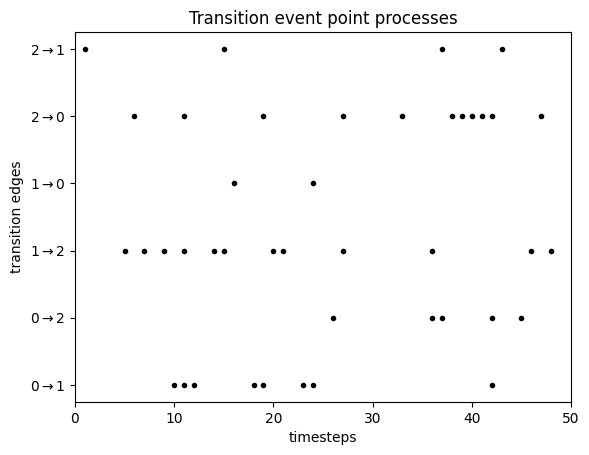
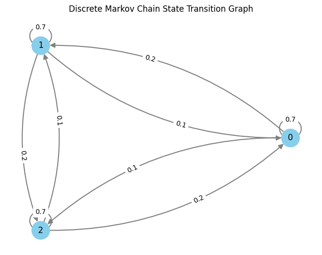
This plot has one line for each transition from a state $i$ to another state $j$. For each of these we drew transition points from a point process. Notice how some of the lines are denser - this is because the corresponding transition probabilities are higher. This is the transition matrix I used:

To turn this set of point processes into a Markov chain, we have to repeat the following steps starting from time 0.

Assume at time $t$ the Markov chain is in state $i$. We consider the point processes for all transitions out of state $i$, and look at the earliest event in any of these sequences that happen after time $t$. Suppose this earlier event is at time $s+t$ and happens in the point process we drew for transition $i \rightarrow j$. Our process will then stay in state $i$ until time $s+t$, then we jump to to state $j$ and repeat the process.

This is illustrated in the following figure:

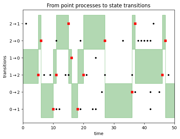
We start the Markov chain in state $1$. We therefore focus on the transitions $1\rightarrow 0$ and $1 \rightarrow 2$, as highlighted by the green area on the left side of this figure. We stay in state $1$ until we encounter a transition event (black dot) for either of these two transitions. This happens after about 5 timesteps, as illustrated by the red cross. At this point, we transition to state $2$, since the first transition event was observed in the $1 \rightarrow 2$ row. Now we focus on transition events for lines $2\rightarrow 1$ and $2\rightarrow 0$, i.e. the top two rows. We don't have to wait too long until a transition event is observed, triggering a state update to state $0$, and so on. You can read off the Markov chain states from where the green focus area lies.

This reparametrisation of a CTMC in terms of underlying Poisson point processes now opens the door for us to simulate non-homogeneous CTMCs as well. But, as this post is already pretty long, I'm not going to tell you here how to do it. Let that be your homework to think about: Go back to process 2 and process 3 of simulating the homogeneous Poisson process. Think about what makes them homogeneous (i.e. the same over time)? Which components would change if the rate matrix wasn't constant over time? Which representation can handle non-constant rates more easily?

Summary

In this post I attempted to convey some crucial, and I think cool, intuition about continuous time Markov chains. I focussed on exploring different representations of a Markov chain, each of which suggest a different way of simulating or sampling from the same process. Here is a recap of some key ideas discussed:

• You can reparametrise a homogeneous discrete Markov chain in terms of waiting times sampled from a geometric distribution, and transition probabilities.
• The geometric distribution has a memory-less property which has a deep connection with the Markov property of Markov chains.
• One way to go continuous is to consider a continuous waiting time distribution which preserves the memorylessness: the exponential distribution. This gave us our first representation of a continuous-time chain, but it's difficult to extend this to non-homogeneous case where the rate matrix may change over time.
• We then discussed different representations of discrete point processes, and noted (although did not prove) their equivalence.
• We could consider continuous versions of these point processes, by replacing discrete distributions by continuous ones, again preserving crucial features such as memorylessness.
• We also discussed how a Markov chain can be described in terms of underlying point processes: each state pair has an associated point process, and transitions happen when a point process associated with the current state "fires".
• This was a redundant representation of the Markov chain, inasmuch as most points sampled from the underlying point processes did not contribute to the state evolution at all (in the last figures, most black dots lie outside the green area, so you can move their locations without effecting the states of the chain).