Connection between denoising and unsupervised learning

This is just a note showing the connection between learning to remove additive Gaussian noise and learning a probability distribution. I think this connection highlights why learning to denoise is, in fact, a form of unsupervised learning. This is despite the fact that the training procedure is more similar to supervised learning and is based on minimising squared loss.

I couldn't find the paper that describes this from the beginning, so I'd rather write this down. People whose work is very relevant to this area are Harri Valpola, Pascal Vincent and colleagues.

Let's for sake of simplicity consider denoising a single dimensional quantity $x$. $x$ has distribution $p_x$, which is unknown to us, but we have i.i.d. samples $x_i$ provided. Let's consider the problem removing additive noise, let $\tilde{x} = x + \epsilon$ denote the noise corrupted version of $x$, where $\epsilon \sim \mathcal{N}(0,\sigma_n) = p_{noise}$. Our aim is to find a denoising function $f$ that reconstructs $x$ from $\tilde(x)$ optimally under the mean squared loss:

$$MSE(f) = \mathbb{E}_{x,\tilde{x}}(x - f(\tilde{x}))^2.$$

It's interesting to think about what this function looks like in the 1D case. Here is a nice illustration from (Rasmus et al):

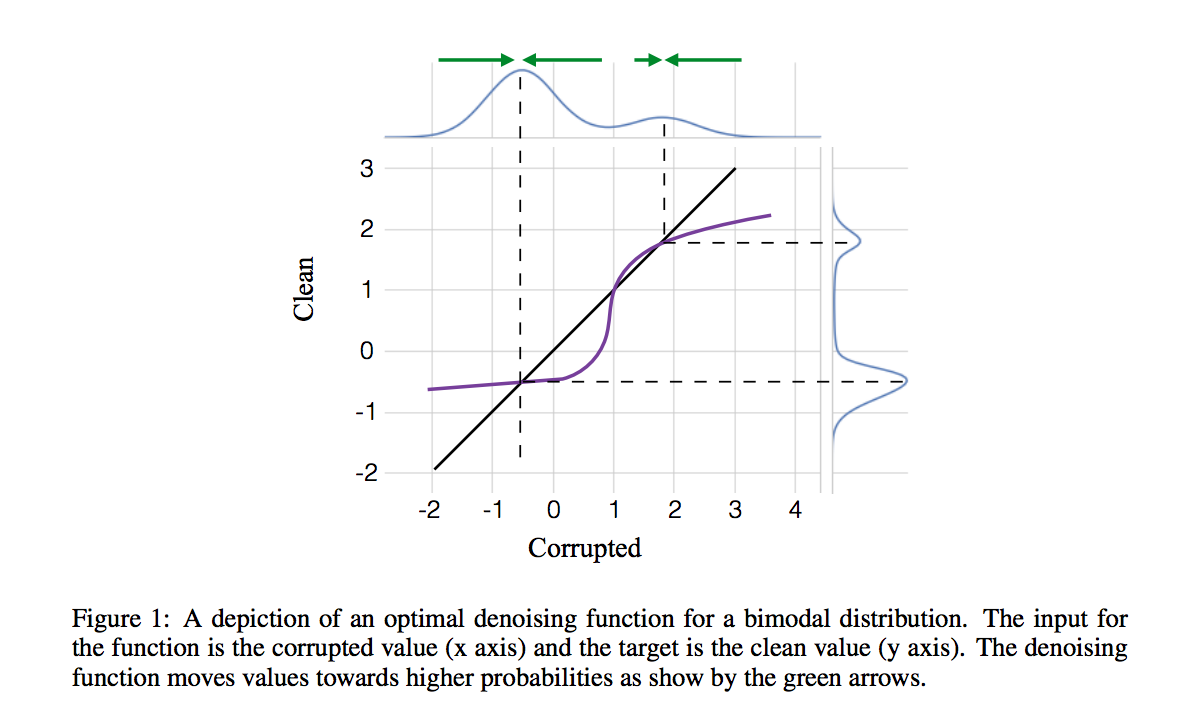
The optimal denoising function

We know that if $f$ can take an arbitrary shape, the optimal solution is the mean of the Bayesian posterior:

$$f^{*}(\tilde{x}) = \mathbb{E}_{x\vert \tilde{x}} [x] = \frac{\int x \cdot p_{noise}(\tilde{x}\vert x) p_x(x) dx}{\int p_{noise}(\tilde{x}\vert x) p_x(x) dx} $$

To reiterate, if we use the MSE to measure reconstruction loss, the Bayesian posterior mean $f^{*}$ is always the optimal reconstruction function. Any method of obtaining a denoising function $f$ by optimising MSE will approximate the performance of the Bayesian optimum, and will have at least the MSE of $f^{*}$.

Approximation for small $\sigma_n$

If the noise variance is low, we can approximate $f^{*}$ analytically by using a locally linear Tailor expansion of the prior distribution $p_x$ around the noise-corrupted observation $\tilde{x}$:

$$p_x(x) \approx p_x(\tilde{x}) + \partial_{x}p_x(\tilde{x}) \cdot (x - \tilde{x})$$

We can substitute this approximation back to the formula for $f^{*}$, and solve the integrals analytically (it's all Gaussians and linear functions so it's easy). The final formula we obtain is:

$$f^{*}(\tilde{x}) \approx \tilde{x} + \sigma^2_{n}\cdot \frac{\partial_{x}p_x(\tilde{x})}{p_{x}(\tilde{x})} = \tilde{x} + \sigma^2_n \cdot \partial_x \log p_x(\tilde{x})$$

So the optimal denoising function is mainly driven by the gradient of the log probability $p_x$ at the corrupted input $\tilde{x}$. This approximation holds anytime where $p_x$ is relatively slowly varying within the lengthscale of the noise distribution.

Observations:

• the denoising function reduces to identity (i.e. f^{*}(\tilde{x})=\tilde{x}) at local optima (or in higher dimensions at saddle points) of the distribution $p_x$. This can also be seen at the figure above. This means that if one runs an iterative denoising procedure by recursively applying $f^{*}$ on the denoised values, the stable fixed points of this process will be the modes (or saddle points) of $p_x$. This raises an interesting question: how about recursively applying denoising starting from the bicubic
• denoising is connected to score matching (see e.g. Pascal Vincent's technical report which is an unsupervised learning method in which the objective function is $\partial_x \log p_x(\tilde{x})$. This derivation highlights why denoising is intimately related to this quantity.
• the optimal denoising function depends trivially on the noise variance $\sigma^2_n$. This means that as long as the noise is small, the denoising function learnt for one noise level can be easily transferred/adapted to work well for a different noise level without additional learning. This only works with Gaussian noise, and the approximation does not hold for large levels of noise.
• when denoising images, or other natural signals, the distribution $p_x$ is high dimensional, highly multimodal, probaby fast changing and concentrated on a manifold. It may not even be smooth or differentiable with respect to pixel values. The smoothness assumptions here are probably violated so the analogy doesn't hold. But dispite this, I think generally it still makes sense to think about denoising as a form of density estimation, and indeed denoising autoencoders have a good motivation from the perspective of manifold learning.