
Comment on "Overcoming catastrophic forgetting in NNs": Are multiple penalties needed?
This comment on the DeepMind folks' latest PNAS paper on overcoming catastrophic forgetting. I liked this paper a lot, I recommend it. Despite this, the post eventually turned into a critical review of the method, rather than the glowing, enthusiastic review I sat down to write. Please don't let this prevent you from reading the paper:
- James Kirkpatrick et al (2017) Overcoming catastrophic forgetting in neural networks, PNAS
First, it's a nice paper: simple, clean, statistically motivated solution (see more on this later) and you can clearly see where this is going and how it's relevant to DeepMind's pursuit of general learning machines. 👏. Second, it's a great achievement of the authors and the community that we now regularly see purely machine learning papers solving a machine learning problems in general journals like PNAS, Science and Nature.
Summary of this post
- I focus on the statistical techniques behind the proposed approach, elastic weight consolidation (EWC), which is best described as on-line sequential (diagonalised) Laplace approximation
- Bayesian inference wouldn't suffer from catastrophic forgetting which haunts optimisation-based methods
- EWC approximates Bayesian computation
- then I look at what happens moving on to the third task. This detail is somewhat glanced over in the paper.
- applying the methodology consistently, I arrive at a formula which is inconsistent with the paper on how the third task is learned.
- the paper suggests keeping multiple parameters and penalties around from all previously learnt tasks, but I think only the latest parameter should be kept as it already implicitly captures all previous tasks.
- keeping multiple quadratic penalties from previous tasks might actually hurt the method's ability to learn new tasks, and results in EWC disproportionately favouring tasks learnt early on
- keeping a single quadratic penalty would also eliminate the need to know what task is currently being performed - although a smart solution for this may help agent performance.
High level overview
Take home message: Bayesians never forget (catastrophically)
There are situations when you want to use the same neural net to solve a range of different tasks. This is not usually a problem if you can afford to train the network on all the tasks simultaneously. The catastrophic forgetting problem arises, however, when you want to train the network to perform new tasks sequentially. How do you train the network on the $k+1$st task without it forgetting everything it knew about the first $k$ tasks?
The authors observe that the catastrophic forgetting does not happen when the network parameters are learnt in a fully Bayesian way. Instead of obtaining single parameter estimate $\theta$ via gradient descent, we really want to maintain a full Bayesian posterior distribution $p(\theta\vert \mathcal{D}_{T_1}, \ldots \mathcal{D}_{T_k})$ over possible parameter values that worked well in previous tasks $T_1 \ldots T_k$. Then we could simply use this posterior as a prior when solving the $k+1$st task $T_{k+1}$ and obtain an updated posterior which captures all tasks $T_1 \ldots T_{k+1}$
Of course, maintaining a full posterior is intractable, and even approximating it can be pretty tricky. How do we bridge the gap between the statistical awesomeness of Bayesian inference and the sheer efficiency of gradient descent? The authors opt for a on-line diagonalised Laplace approximation approach, which they call elastic weight consolidation (EWC). The approach is similar to assumed density filtering (ADF, Opper & Winther, 1999), which is a precursor to expectation-propagation (Minka, 2001), a connection highlighted by the authors.
Laplace approximation
Laplace approximation takes a probability density $p$ and approximates it with a Gaussian, whose mean is at the mode of the distribution and variance is given by the inverse Hessian of the log density $\log p$ at the mode. This approximation to Bayesian posteriors is motivated by Bernstein-von Mises-type convergence theorems which state that in identifiable exchangeable models the posterior will converge to the Laplace. EWC uses a diagonalised Laplace approximation, which ignores the off-diagonal entries of the Hessian and keeping only diagonal ones. Applied to neural networks, the diagonal assumption is the same as saying that the parameters of the network have completely independent influence on the loss function (which is of course not true, but perhaps true enough).
The elastic weight consolidation (EWC) method proposed in the PNAS paper essentially applies Laplace approximation recursively, in an on-line fashion, learning one task after another with a neural network.
Diving deeper
Let's look at what precisely the EWC algorithm does.
Learning a second task after the first
This is the easier case. Let's follow the footsteps of the authors, with a slight change in notation. The posterior of NN parameters $\theta$ given the first two tasks $A$ and $B$ can be decomposed as follows:
$$
\log p(\theta\vert \mathcal{D}_A, \mathcal{D}_B) = \log p(\mathcal{D}_B\vert \theta) + \log p(\theta\vert \mathcal{D}_A) - \log p(\mathcal{D}_B\vert \mathcal{D}_A)
$$
The left-hand term is the log likelihood, or task-specific objective function for task $B$, the right-hand term can be thought of as an adaptive elastic weight regularizer that tries to maintain knowledge of the first task. I think there's an irrelevant typo in the paper: the last term of Eqn. (2) should be $\log p(\mathcal{D}_B\vert \mathcal{D}_A)$ rather than $\log p(\mathcal{D}_B)$. It doesn't matter as it's constant w.r.t. $\theta$ anyway.
$\log p(\theta\vert \mathcal{D}_A)$, of course, is intractable to compute, so we're going to approximate it with a diagonalised Laplace approximation. For this we need the mode $\operatorname{argmax}_\theta \log p(\theta\vert \mathcal{D}_A)$ and the Hessian of $\log p(\theta\vert \mathcal{D}_A)$ evaluated at the mode.
The mode $\theta^A$ can be found via usual gradient descent, minimising the loss $\mathcal{L}_A(\theta) - \log p(\theta)$, where the prior $p(\theta)$ acts as a regulariser. (the authors don't actually use a prior so ignore that term). The Hessian will be the sum of the Fisher information from task $A$ which I denote $F^A$, plus the Hessian of the log prior $\log p(\theta)$ (which, again, the paper doesn't have. This is no big deal as the prior would probably be a dummy weak regulariser anyway).
So, substituting these back to a diagonalised Laplace approximation we obtain:
$$
\log p(\theta\vert \mathcal{D}_A, \mathcal{D}_B) \approx -\mathcal{L}_B(\theta) - \frac{1}{2}\sum_i F^A_{i,i} (\theta_i - \theta^A_i)^2 + \text{constant}
$$
where $\mathcal{L}_B$ is the negative log likelihood, or loss function, of task $B$, and the Gaussian approximation to $p(\theta\vert \mathcal{D}_A)$ acts as a nice quadratic regulariser, which is dependent on data from task $A$. The authors also introduce $\lambda$, an importance weight which I will assume is $1$ to keep things simple.
We can now train our network via our favourite gradient descent technique solving the following optimisation:
$$
\theta^{A,B} = \operatorname{argmin}_\theta \mathcal{L}_B(\theta) + \frac{1}{2}\sum_i F^A_{i,i} (\theta_i - \theta^A_i)^2
$$
Pretty cool. We have a data-dependent $L_2$ regulariser which adapts to task $A$ we already learnt about. This regulariser captures our knowledge of task $A$, so we can now focus on the new task $B$, while the regulariser makes sure we don't catastrophically forget about $A$. Makes sense.
As a result, $\theta^{A,B}$ will be a parameter that has good performance on both $A$ and $B$.
Learning the third task after the first two
On moving to the third task, the authors say only this:
When moving to a third task, task C, EWC will try to keep
the network parameters close to the learned parameters of both tasks A and B. This can be enforced either with two separate penalties or as one by noting that the sum of two quadratic penalties is itself a quadratic penalty
🤔
Do we actually need to remember $\theta^A$? $\theta^{A,B}$ is supposed to be the mode of the posterior $p(\theta\vert \mathcal{D}_A, \mathcal{D}_B)$ and the posterior already captures all our knowledge about both tasks $A$ and $B$. The mode of the previous posterior $\theta^A$ should become irrelevant as it is already incorporated into $\theta^{A,B}$. Somehow, this just doesn't feel right.
Let's apply the sequential diagonal Laplace approximation argument consistently, but now for learning the third task $C$, after $A$ and $B$. For this, we need the mode and Hessian of the posterior $p(\theta\vert \mathcal{D}_A, \mathcal{D}_B, \mathcal{D}_C)$, which can be expressed as:
$$
\log p(\theta\vert \mathcal{D}_A, \mathcal{D}_B, \mathcal{D}_C) = -\mathcal{L}_C(\theta) + \log p(\theta \vert \mathcal{D}_A, \mathcal{D}_B) + \text{constant}
$$
Let's replace the intractable $\log p(\theta \vert \mathcal{D}_A, \mathcal{D}_B)$ with its Laplace approximation, once again. We have already calculated the mode of this distribution, it is (approximately) $\theta^{A,B}$. How about its Hessian around $\theta^{A,B}$? Well, we have assumed that
$$
\log p(\theta \vert \mathcal{D}_A, \mathcal{D}_B) \approx - \mathcal{L}_B(\theta) - \sum_i F^{A}_{i,i} (\theta_i -\theta^A_i)^2 + \text{constant}
$$
so the Hessian is the Fisher information matrix $F^{B}$ plus the previously assumed diagonal approximation $diag(F^{A})$. So, if we plug these in to form a diagonal Laplace approximation to $\log p(\theta\vert \mathcal{D}_A, \mathcal{D}_B)$, we get:
$$
\log p(\theta\vert \mathcal{D}_A, \mathcal{D}_B) \approx - \sum_i (F^{A} + F^{B})_{i,i} (\theta_i - \theta^{A,B}_i)^2 + \text{constant}
$$
Using this approximation, the optimisation problem for task $C$ after tasks $A$ and $B$ have been learnt will look like:
$$
\theta^{A,B,C} = \operatorname{argmin}_\theta \mathcal{L}_C + \sum_i (F^{A} + F^{B})_{i,i} (\theta_i - \theta^{A,B}_i)^2
$$
Note that there is just a single penalty, and it is around $\theta^{A,B}$ which is the parameter we learnt for task $B$ while regularising for not forgetting task $A$. We don't need a second penalty term around $\theta^A$ as it's already been taken into account when finding $\theta^{A,B}$. $\theta^{A}$ is now irrelevant and we can throw it away. $\theta^{A,B}$ (approximately) captures both tasks $A$ and $B$. All we need to do is update the regulariser's weights to $F^{A,B}_{i,i} := (F^{A}_{i,i} + F^{B})_{i,i}$.
So, let's contrast this with what the paper says: "When moving to a third task, task $C$, EWC will try to keep the network parameters close to the learned parameters of both tasks A and B. This can be enforced either with two separate penalties or as one by noting that the sum of two quadratic penalties is itself a quadratic penalty."
I don't think this is the correct approach. There are a few possible explanations, in the order of my preference:
- I made a mistake here and my derivation is wrong
- the authors use a different reasoning from mine to derive multiple, task-specific penalties for the third task, in which case I'd be curious to hear that
- the paper described what is actaully done ambiguously in the text, and they actually do the right thing when implementing EWC
- the authors made a mistake, and if this is the case the algorithm may be further improved by fixing the mistake
Why would multiple penalties be wrong?
Let's see what happens if you do keep the two penalties around, one centered around $\theta^A$ and one around $\theta^{A,B}$? In a handwavy way, it corresponds to optimising something a bit - but not quite - like this:
$$
-\mathcal{L}_{C} + \log p(\theta\vert \mathcal{D}_A, \mathcal{D}_B) + \log p(\theta\vert \mathcal{D}_A)
$$
Not only does this formula not add up from Bayes' rule's perspective, it also places too much emphasis on task $A$, more than what Bayes' rule would warrant. Furthermore, as more tasks are added, task A will be overemphasized further. Therefore, I think
keeping multiple penalties around might result in a diminished ability to learn new tasks, as early tasks get disproportionately more weight.
In a thought experiment, imagine what would happen if $\mathcal{L}_{C}$ were completely flat, that is, you want to learn task $C$, but you have no actual data, or the data provides no information about $\theta$ (I know, stupid assumption, but makes sense to think about it). Let's run gradient descent on the penalised loss nevertheless, essentially minimising only penalty term(s).
If you have the one penalty around the most recently learned parameter $\theta^{A,B}$, as in my derivation, then $\theta^{A,B}$ is already the minimum. If task $C$ has no new data, you just don't change your parameters from what you had before. Makes sense, right? If it's not broken, why fix it?
However, if you have the two penalties, one around $\theta^{A,B}$, and one around $\theta^A$, your optimisation will actually move away from $\theta^{A,B}$, back towards $\theta^A$ a bit. But this would make no sense at all. Why would you change the parameters if you are presented with no new evidence at all?
For the South Park afficionados out there: the extra penalties are basically member berries. They will make your network want to go back to the old ways when it solved task $A$ perfectly and everything seemed so easy.

Does it actually appear to hurt the algorithm?
Well, not really. At least it's hard to tell from the Figures. Look at Figure 3.A:
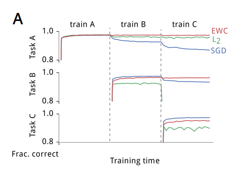
This shows that while EWC very successfully retains its performance at task $A$, the gap between SGD and EWC on new tasks widen. How would the harmful effects of keeping two penalties around show up on this Figure?
- Performance on Task $A$ first goes down a bit after training for a few new tasks, but then eventually gradually goes up again as we train for tasks $E,F\ldots$. This would happen because as time goes by, you implicitly add the 'Task A' penalty over and over again, even though that penalty is implicitly captured in all other task penalties as well. We can't really see this effect here, partly because the performance on task A never really drops, and partly because it only shows 3 tasks. Plus, a lot of this depends on how the $\lambda$ values were chosen, too.
- The gap between EWC and SGD for Task B would be much smaller than the gap between EWC and SGD for Task C. Again, it's hard to say if this is the case or not from this figure.
Similarly, looking at Figure 3.B doesn't really help us analyse if the mismatch in penalties causes any problems, because we only see average task performance.
Do you even need to know what task you're performing?
This is what the authors write about the need to identify the task being performed:
Inspired by this evidence, we augmented the DQN agents with
extra functionality to handle switching task contexts. Knowledge of which task is being performed is required for the EWC algorithm as it informs which quadratic constraints are currently active and also which quadratic constraint to update when the task context changes.
Now, good news is that knowledge of task identity may not be a requirement for the algorithm to work after all. If there are no task-specific quadratic penalties, only a single one, we don't have to choose betwen them. We can just update the single posterior mode $\theta^{A,\ldots}$ and the Hessian $F^{A,\ldots}$ in an on-line fashion and forget their old values.
sidenote: In fact, EWC with a single quadratic penalty could be applied more generally than the catastrophic forgetting problem. There is nothing in the derivation that specifies that $\mathcal{D}_A$ and $\mathcal{D}_B$ should in fact correspond to two different tasks. They can even contain data from different tasks, so we don't even need to synchronise the freezing of the quadratic penalty with swittching tasks.
Or, $\mathcal{D}_A,\mathcal{D}_B,\ldots$ can be minibatches of data from a single task, in which case EWC can be thought of as an on-line alternative to stochastic gradient descent. Consider looping through the minibatches one-by-one. On each minibatch, instead of doing a single gradient step like in SGD, we run full gradient descent with a quadratic regulariser until convergence. Once converged, we update the quadratic regulariser according to the Laplace rules, and load the next minibatch. This may not be as accurate as SGD because of the diagonal Laplace approximation introduces inaccuracies over time. But it would require less overall data shoveling between GPU memory and main memory, and it accesses each minibatch exactly once. So there might be situations when such algorithm would be a meaningful alternative to SGD.
Of course, the agent performing the tasks will probably still benefit from an elaborate mechanism to detect task identity, but that is a different concern entirely. The point is, the algorithm at a computational level is agnostic to tasks beyond evaluating the loss functions $\mathcal{L}_A,\mathcal{L}_B,\ldots$
Summary
This is a great paper, and a great demonstration of how a simple, statistically motivated algorithm can make a huge difference.
I did, honestly, set out to write a very positive review, I really liked the statistical motivation, and the resulting simplicity of the method. The experiments are also interesting and well done, the results speak for themselves. It is also exciting to think about how this can be used in practice, and being able to learn tasks sequentially is bound to have a massive impact.
But look at the post now: at best, I'd describe it as constructive criticism, I ended up zooming in on the one thing that wasn't quite kosher, even though you can hardly argue with the performance of the method. But this is also a good motivation for continuing to write these posts: had I not started trying to explain how and why the method works, I may have missed this entirely. And then, of course, it is entirely possible that the authors actually did the same thing I describe here, just explained it in a different way, or that there are alternative justifications for the multiple penalties approach.