
The Blessings of Multiple Causes: Causal Inference when you Can't Measure Confounders
Happy back-to-school time everyone!
After a long vacation (in blogging terms), I'm returning with a brief paper review which conveniently allows me to continue to explain a few ideas from causal reasoning. Since I wrote this intro to causality, I have read a lot more about it, especially how it relates to recommender systems.
Here are the two recent papers this post is based on:
- Yixin Wang and David Blei (2018) The Blessings of Multiple Causes
- Yixin Wang, Dawen Liang, Laurent Charlin and David Blei (2018)
The Deconfounded Recommender: A Causal Inference Approach to Recommendation
UPDATE: After publishing this post, commenters pointed me to excellent in-depth blog posts by Alex d'Amour on the limitations of these techniques: on non-identifiability and positivity. I recommend you go on and read these posts if you want to learn more about the conditions in which the proposed methods work.
Summary
- I'll set the scene by revisiting the basic example of Simpson's paradox, a great illustration of confounders.
- I will then talk about the practice of controlling for confounders, and the limitations of the approach
- Wang and Blei (2018) consider the case when you can't identify and/or measure all the confounders
- the core of the idea is to construct a "substitute confounder" by fitting a factor model to the join distribution of multiple cause variables
- if our model is correct, this substitute confounder is guaranteed to contain all information about all actual confounders which influence at least two of the cause variables
- finally, I talk a bit more about the assumptions and limitations of the work
Example: Simpson's paradox
Simpson's paradox is a commonly used example to introduce confounders and how they can cause problems if not handled appropriately. I'm going to piggyback on the specific example from (Bottou et al, 2013), another excellent paper that should be on your reading list if you haven't read it already. We're looking at data about the success rate of two different treatments, A and B, for kidney stone removal:
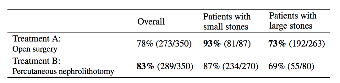
Look at the first column "Overall" first. The average success rate of treatment A is 78%, while the success rate of treatment B is 83%. You might stop here and conclude that treatment B is better because it's successful in a higher percentage of cases, and continue recommending treatment B to everyone. Not so fast! Look at what happens if we group the data by the size of kidney stone. Now we see that in the group of patients with small stones, treatment A is better, in the group with large stones we also see that treatment A is better. How can treatment A be superior in both group of patients, but treatment B be better overall?
The answer lies in the fact that patients weren't randomly allocated to treatments. Patients with small stones are more likely to be assigned treatment B. These are also patients who are more likely to recover whichever treatment is used. Coversely, when the stone is large, treatment A is more common. In these cases the success rate is lower overall, too. Therefore, when you group data from the two groups, you ignored the fact that the treatments were assigned "unfairly", in the sense that treatment A was on average assigned to many more patients who had a worse outlook to begin with.
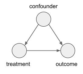
In this case, the size of the kidney stone is a confounder variable. A random variable that causally influences both the assignment of treatments, and the outcome. Graphically, it looks like this:
Controlling for Confounders
If we use $T, C$ and $Y$ to denote the treatment, confounder and the outcome respectively, and denote treatments A and B as 0 and 1, this is how one could correctly estimate the causal effect of the treatment on the outcome, while controlling for the confounder $C$:
$$
\mathbb{E}_{c\sim p_C}[\mathbb{E}[Y\vert T=1,C=c]] - \mathbb{E}_{c\sim p_C}[\mathbb{E}[Y\vert T=0,C=c]]
$$
Or, alternatively, with the do-calculus notation:
$$
\mathbb{E}[Y\vert do(T=1)] = \mathbb{E}_{c\sim p_C}[\mathbb{E}[Y\vert T=1,C=c]]
$$
Let's decompress this. $\mathbb{E}[Y|T=0,C=c]$ is the average outcome, given that treatment $1$ was given and the confounder took value $c$. Simple. Then, you average this over the marginal distribution of the confounder $C$.
Let's look at how this differs from the non-causal association you would measure between treatment and outcome (i.e. when you don't control for $C$:
$$
\mathbb{E}[Y\vert T=1] = \mathbb{E}_{c\sim p_{C\vert T=1}}[\mathbb{E}[Y\vert T=1,C=c]]
$$
So the two expressions differ in whether you average over $p_{C\vert T=1}$ or $p_{C}$ in the right-hand side. How does ethis expression come about? Remember from the previous post that the effect of an intervention, $do(T=1)$, can be simulated in the causal graph by severing all edges that point into the variable we intervene on. In this case, we sever the edge from the confounder $C$ to the treatment $T$ as that is the only edge pinting to $T$. Therefore, in the alternative model where the link is severed, $C$ and $T$ become independent and thus $p_{C\vert do(T=1)} = p_{C}$. Meanwhile, as no links leading from either $C$ or $T$ to $Y$ have been severed $p(Y\vert T, C)$ remains unchanged by the intervention.
What can go wrong?
So, if correcting for confounders is so simple, why is it not a solved problem yet? Because you don't always know the confounders, or sometimes you can't measure them.
Controlling for too little: You may not be measuring all confounders. Either because you're not even aware of some, or because you're aware of them but genuinely can't measure their values.
Controlling for too much: You may be controlling for too much. When one wants to make sure all confounders are covered, it's commonplace to simply control for all observable variables, in case they turn out to be confounders. This can go wrong, or very wrong. In ML terms, every time you control for a confounder, you add an extra input to the model to approximate $P_{y\vert T, C}$, increasing complexity of your model, likely reducing its data efficiency. Therefore, if you include a redundant variable in your analysis as a confounder, you're just making your task harder for no additional gain.
But, even worse things can happen if you include the a variable in your analysis which you must not condition on. Mediator variables are ones whose value is causally influenced by the treatment, and they causally influence the outcome. In graph notation, it is a directed chain like this: $T \rightarrow M \rightarrow Y$. If you control for mediators as if they were confounders, you are shielding the causal effect of $T$ on $Y$ via $M$, so you are going to draw incorrect conclusions. The other situation might be conditioning on a collider $W$, which is causally influenced by both the treatment, and the outcome $Y$, i.e. $T \rightarrow W \leftarrow Y$. If you condition on $W$, the phenomenon of explaining away occurs, and you induce spurious association between $T$ and $Y$, and again, you draw incorrect conclusions. A common, often unnoticed, example of conditioning on a collider is sampling bias, when your datapoints are missing not at random.
In general case, given a causal model of all variables in question, do-calculus can identify the minimal set of variables you have to measure and condition on to obtain a correct answer to your causal query. But in many applications, it we simply don't have enough information to name all the possible confounding factors, and often, even if we suspect the existence of a specific confounder, we won't be able to measure or directly observe it.
The Blessings of Multiple Causes
Wang and Blei (2018) address this problem with the following idea: instead of identifying and then measuring possible confounders, let's try to automatically discover and infer a random variable which can act as a substitute confounder in our analysis.
This is possible in a special setting when:
- there are multiple cause variables $A_{i,j}$, also called assignment variables. Imagine a setup where patients can receive multiple treatments (or any combination of them), and each of the treatments may have a causal effect on the outcome. Essentially, in our previous graph, imagine that $T$ is a multivariate vector.
- there may be confounders, but all confounders causally influence at least two of the cause variables. I.e. we assume that there are no single-cause confounders which only influence one of the treatment variables and the outcome, but is otherwise causally unrelated to the other treatments
- the cause variables are distributed according to a latent factor model (which we can approximate and learn from data).
In a latent factor model (like matrix factorization, PCA, etc) the user-treatment matrix is modeled by two sets of random variables: one for each treatment, one for each user. A general factor model structure is shown below:
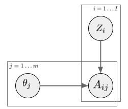
$A_{i,j}$ is the assignment of treatment $j$ to data instance $i$. We can imagine this as binary. Its distribution is determined by the instance-specific random variable $Z_i$, and the treatment-specific $\theta_j$. The key observation is, as we look across instances $i$, conditioned on the $Z_i$ vector, the treatment assignments $A_{i,j}$ become conditionally independent between treatments $j$. It is this $Z_i$ variable which will be used as a substitute confounder. Figure 1 of the paper illustrates why:
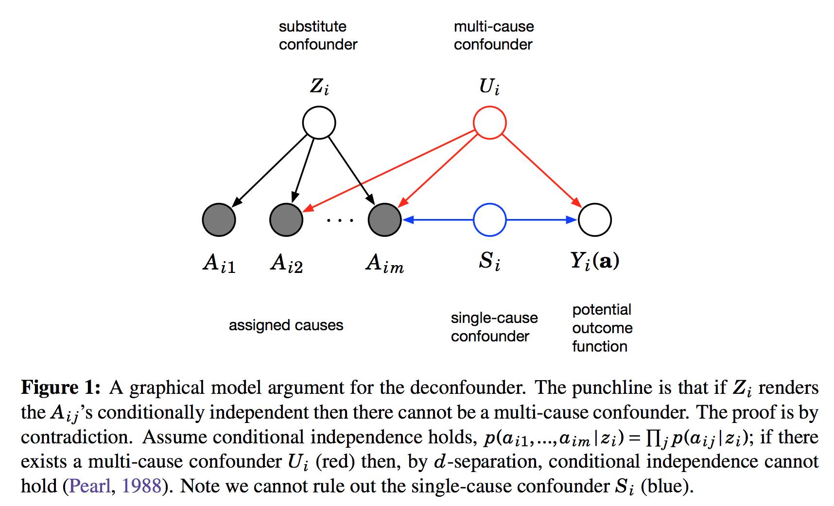
This figure shows the graphical structure of the problem. For the instance $i$ we have the $m$ different assignments $A_{i1}\ldots A_{im}$ and the outcome $Y_i$. Causal arrows between the assignments $A$ and the outcome $Y$ are not shown on this Figure but it is assumed some of them might exist. We also calculate the latent variable $Z_i$ and call it substitute confounder. As $Z_i$ renders the otherwise dependent $A$s conditionally independent it appears as a common parent node in this graph. The argument is the following: if there was any confounder $U_i$ which effects multiple assignment variables simultaneously, it must either be contained within $Z_i$ already (which is good), or our factor model cannot be perfect. Incorporating $U$ as part of $Z$ would improve our model of $A$s.
Therefore, we can force $Z_i$ to incorporate all multi-cause confounders by simply improving the factor model. Sadly, this argument relies on reasoning about marginal and conditional independence between the causes $A$, so it cannot work for single-cause confounders.
In a way this method, called the deconfounder algorithm, is a mixture of causal discovery (learning about structure of the causal graph) and causal inference (making inferences about variables under interventions). It identifies just enough about the causal structure (the substitute confounder variable) to then be able to make causal inferences of a certain type.
Limitations
The obvious limitation of this method - and the authors are very transparent about this - is that it cannot deal with single-cause confounders. You have to assume if there is a confounder in your problem, you will be able to find another cause variable causally influenced by the same confounder in order to use this method.
The other limitation is the assumption that the assignments follow a factor model distribution marginally. While this may seem like a relatively OK assumption, it rules a couple of interesting cases out. For example, the assumption implies that the treatments cannot directly causally influence each other. In many applications this is not a reasonable assumption. If I make you watch Lord of the Rings it will definitely causally influence whether you will want to watch Lord of the Rings II. Similarly, some treatments in hospitals may be given or ruled out because of other treatments.
Finally, while the argument guarantees that all multi-cause confounders will be contained in the substitute confounder, there is no guarantee that the method will identify a minimal set of confounders. Indeed, if there are factors which influence multiple $A$s but are unrelated to the outcome, those variables will be covered by $Z$ as well. It is not difficult to create toy examples where the majority of the information captured in $Z$ is redundant.
Deconfounded Recommender
In the second paper, Wang et al (2018) use this method to the specific problem of training recommender systems. The issue here is that vanilla ML approaches work only when items and users are randomly sampled in the dataset, which is rarely the case. Whether you watch a movie, and whether you like it are confounded by a number of factors, many of which you cannot model or observe. The method does apply to this case, and it does better than their but the results lack the punch I was hoping to see.
Nevertheless, this is a very interesting direction, and also quite a bit different from many other approaches to the problem. UPDATE: As it was evident from commenters' reaction to my post, there is a great deal of discussion taking place about the limitations of these types of 'latent confounder identification' methods. Alex d'Amour's blog posts on non-identifiability and positivity go into a lot more detail on these.