
Are Energy-Based GANs any more energy-based than normal GANs?
EDIT: The post had a mistake, pretty crucial one, kindly pointed out by George Tucker, so the has changed from what it was in the original. I have falsely claimed that a variant of the general GAN algorithm is pathological, this turns out not to be the case. Sorry for the mistake.
For our latest reading group I chose to read a paper fresh out of Yann LeCun's lab, it's really just a few days old:
- Junbo Zhao, Michael Mathieu and Yann LeCun (2016) Energy-based Generative Adversarial Network
When I saw the title of the paper and skimmed through the abstract I got pretty excited: finally a paper that takes an energy-based view of GANs rather than "two players playing a game against each other and we're looking for the Nash equilibrium" view. I do think that thinking about energies is the most promising way to understand how and why GANs work and also why they mostly don't work.
As I was reading the paper, my excitement has disappeared somewhat. Instead of a nice theoretical framework I was hoping to see, the authors' choices looked a bit arbitrary to me, loosely motivated by intuition. In this post I'm trying to explain how I think about energy-based GANs (EBGANs). I'm only really going to touch on very big-picture details instead of covering all details of the paper.
Summary of this note
- I introduce a unifying framework to think about GAN-type methods. This includes the original GAN and energy-based EBGANs as special case
- I show different special cases of this general algorithm, using least-squares importance estimation and hinge-loss
- I finally cast the EBGAN objective in this framework
- in this framework, the choices the authors made look rather arbitrary, I don't see why this particular algorithm should do well, and I find it hard to predict the behaviour of the algorithm compared to regular GANs
A unifying view on GAN-type algorithms
Here is a unifying framework I use to think about some GAN-style algorithms in general. We have some generative model $Q$, which we can sample from easily. We want to fit this to data sampled from $P$. I think about GANs as an inner loop and outer loop (even though this is not how they're often implemented):
- inner loop: we train a discrepancy function $s(x)$ to - generally speaking - assign high values to fake data $x\sim Q$, and low values to real data $x\sim P$. We do this using a loss function $\mathcal{L}(s;P,Q)$, or just $\mathcal{L}(s)$ for short. This loss usually takes the following separable form:
$$
\mathcal{L}(s;P,Q) = \mathbb{E}_{x\sim P}\ell_1(s(x)) + \mathbb{E}_{x\sim Q}\ell_2(s(x)),
$$
where $\ell_1$ and $\ell_2$ are scalar penalties applied on the value of $s$ over real and fake examples respectively (we'll see concrete examples below). Let's call the optimal discrepancy function for the current $Q$
$$
s^{\ast} := \operatorname{argmin}_s \mathcal{L}(s,P,Q)
$$
where I omit the dependence of $s^{\ast}$ on $Q$ and $P$ in the interest of brevity. - outer loop: we take a gradient step to update the generator $Q$ by trying to decrease the average value of the optimal discrepancy function for generated samples $\mathbb{E}_{x\sim Q} s^{\ast}(x)$. In some variants we instead minimise a monotonic function, $f$ of the discrepancy $\mathbb{E}_{x\sim Q} f(s^{\ast}(x))$.
Intuitively, this class of algorithms make sense: each iteration we improve $Q$ by decreasing the discrepancy between $P$ and $Q$. We can identify different variants of GAN as a special case of this unifying framework by picking the right discriminator loss $\mathcal{L}(s)$ and nonlinearity $f$.
Original GAN: Logistic regression
In the original GAN we train the discrepancy function $s$ by logistic regression. In the original GAN the discriminator $D$ is a classifier, and $s$ is its un-normalised output before the final logistic sigmoid is applied:
$$
D(x) = \frac{1}{1 + e^{-s(x)}}
$$
The training criterion for $s$ becomes the following:
\begin{align}
\mathcal{L}(s) &= \mathbb{E}_{x \sim P} \log D(x) + \mathbb{E}_{x \sim Q} \log (1 - D(x)) \\
&= \mathbb{E}_{x \sim P} \operatorname{softminus}(s(x)) -
\mathbb{E}_{x \sim Q} \operatorname{softplus}(s(x))
\end{align}
These two penalty terms are shown in the figure below:
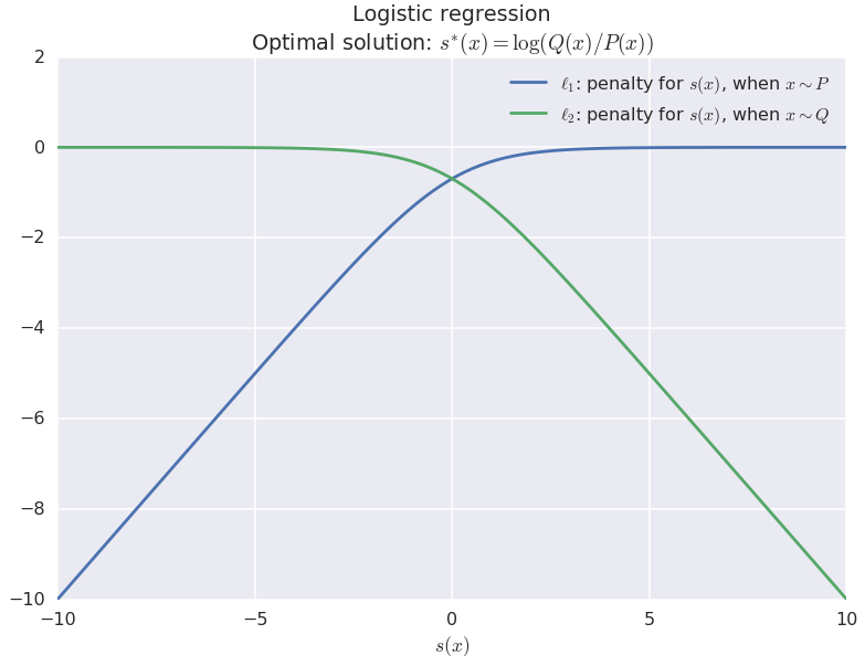
The way to interpret this graph is as follows: $s$ maps our data $x$ onto a scalar, a point on the x-axis. The green curve is the penalty that we incur for fake data: it decreases as $s(x)$ increases, thus pushes $s$ upwards. For real data, the we incur the blue penalty, which pushes pushes $s$ towards lower values. Therefore, the optimal discrepancy function will have the propery we want: it takes lower values for real data, and higher values for fake data.
But we can be even more precise. We know that the optimal discrepancy function for logistic regression is actually the logarithmic probability ratio:
$$
s^{\ast}(x) = \left( \operatorname{argmin}_s \mathcal{L}(s) \right)(x) = \log\frac{Q(x)}{P(x)}
$$
So as we train the discriminator, $s$ is getting closer to this log-ratio.
Here is where energies come in. Usually, by energy of a distribution we mean the negative logarithm of it's probability density function $E_P = -\log P$. Using this definition we can say that the discrepancy function in GANs actually learns the difference of energies:
$$
s^{\ast} = \log Q - \log P = E_{P} - E_{Q}
$$
This is also why it makes sense to minimise the expected discrepancy function $\mathbb{E}_{x \sim Q} s(x)$ when the generator $Q$ is updated: it amounts to minimising $\operatorname{KL}[Q|P]$ as I wrote in an earlier post. Similarly, if we choose nonlinearity $f = \operatorname{softplus}$ in the outer loop, we recover the GAN variant which minimizes Jensen-Shannon-divergence, while choosing $f = \operatorname{softminus}$ recovers the version the authors use in the original paper and in DCGAN.
This also means that
GANs using logistic regression are actually kind of an energy-based method already
However, let's now see what happens if we mess around with the discriminator loss $\mathcal{L}$. The Bayes-optimal $s^{\ast}$ will not always end up as nice as the difference of energies. Let me give you another super-fun example, least-squares importance estimation (Kanamori et al, 2009)
Least-squares importance estimation
Let's consider the following penalty for $s$ in the inner loop:
$$
\mathcal{L}(s) = \mathbb{E}_{x \sim P} s^2(x) - 2 \mathbb{E}_{x \sim Q} s(x) \
$$
These penalties are illustrated in the figure below:
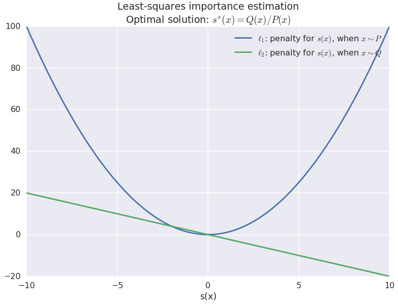
For real data ($x\sim P$) $s$ is anchored to values around $0$ by a quadratic penalty. For fake data, $s$ is pushed up higher (to the right). So again, the intuition holds: $s$ is trained to assign higher values to fake data than to real data, only this time we're using different penalties.
It can be shown that if we train $s$ using this penalty, the Bayes-optimal discrepancy function becomes
$$
s^{\ast}(x) = \frac{Q(x)}{P(x)},
$$
the same as logistic regression but without the logarithm, and this turns out to be a very important difference. For the very simple and intuitive derivation I highly recommend reading (Kanamori et al, 2009).
here is the part where I had a mistake before, thanks again to George Tucker for pointing it out
If you plug that $s^{\ast}$ into the outer loop minimisation, we get the following formula:
$$
\mathbb{E}_{x\sim Q} \frac{Q(x)}{P(x)} = \int Q^{2}(x) P(x) dx
$$
This is similar to the definition of the Rényi $\alpha$-divergence I wrote about last week, except for a missing logarithm. If you choose a nonlinearity $f(x) = x^{\alpha - 2}$, you can recover Rényi divergences for different alpha. The problem is that our minibatch Monte Carlo estimate of the Rényi divergence is going to be biased (for the same reason it is biased in the variational bound case).
Rényi divergences behave differently depending on the choice of $\alpha$ so we should expect that these GAN variants would also differ considerably. See also f-GANs which also use GAN-type algorithms to minimise f-divergences.
EBGANs: "Energy Based" GAN
This brings us to the proposed EBGANs. If you've read the paper, try to ignore the autoencoder aspect for now, I'm going to jump right through equations (1) and (3). What they call $D$ or sometimes the energy, takes the role of our discrepancy function $s$. Substituting $s$ into Eqn. (1) the loss function for training $s$ becomes:
$$
\mathcal{L}(s) = \mathbb{E}_{x \sim P} s(x) - \mathbb{E}_{x \sim Q} (m - s(x))_{+}
$$
The associated penalties are shown in the figure below:
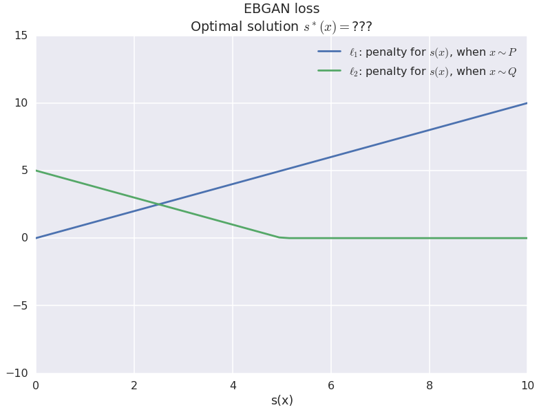
Note that by construction, the authors also restrict $s$ to take non-negative values, so I only show that part of the plot here. The penalty for fake samples (green line) decreases linearly until it hits threshold $m$. So for fake samples $s$ is encouraged to grow, but once you reach the threshold the loss function doesn't care anymore. Simultaneously, the blue penalty encourages $s$ to take lower values when evaluated on real data.
So once again, intuitively it makes sense, the discrepancy function will take higher values for fake data and lower values for real data. Great. But that's basically all I can say. We have no idea, really, what the optimal discrepancy function $s^{\ast}$ would end up looking like. We don't know if it's still as cleanly related to energies $E_P$ or $E_Q$ as it in the logistic regression case - most likely not. The only correct mathematical characterisation of $s^{*}(x)$ I could come up with is this:
$$
s^{*}(x) = \text{¯\_(ツ)_/¯}(x)
$$
So while the paper claims to bridge the gap between GANs and energy-based methods, I actually feel like it's less energy-based than vanilla GANs. The authors interpret $s$ (again, they call it $D$) as an energy function itself, but I don't think it's necessarily an energy function of any meaningful distribution involved. It is related somehow to $P$ and $Q$, and therefore to $E_P$ and $E_Q$, but that dependence is almost certainly nonlinear, and not nearly as clear as in the logistic regression case. In this sense I actually think
normal GANs are slightly more energy-based than Energy-Based GANs.
But what about all the auto-encoder stuff?
The energy-based view of EBGANs is partly motivated by the fact that $D$ is calculated in a special way: it's the mean-squared-reconstruction-error of an autoencoder. As far as I'm concerned, $D$ is just a function that takes a datapoint $x$ and outputs a scalar. I don't see why restricting the architecture would suddenly justify calling $D$ an energy in this case.
True, if the autoencoder in $D$ was trained to perform reconstruction on data sampled from $P$ then, indeed, we could make connections between the reconstruction error and the energy $E_P$. But here, $D$ is trained using a different loss function in $Eqn. (1)$ so any connection that applies when trained on $P$ only is likely not valid anymore. The authors certainly don't provide a proof or formula for what they think the connection between $D$ and $E_P$ or $E_Q$ is.
Summary
There's a lot of hype around GANs these days, and some people feel a lot of it is mostly fluff. I think there are elements of GAN research that, when understood correctly, can become very useful tools in probabilistic modelling. Interpreting GANs in an energy-based or information-theoretic framework is one of those directions.
I had high hopes for this paper, based on its title and a brief skim, but when you consider the details, I don't think it lives up to its title. It does not discuss the implications of choosing different training objectives on the behaviour of the algorithm, other than providing intuition. As we have seen, intuition alone is not enough to predict how the algorithm would work, and a lot depends on the fine details. You have to give credit where credit is due, the paper also has very extensive experiments, in an exhaustive grid-search they ran orders of magnitude more experiments than I have ever done with GANs. And the results to look good, even if they aren't leaps and bounds better than other GAN samples you see these days.
Fineprint: I review papers I read, and from time to time these reviews come out negative. It seems like this is that time of the year again... It's the second negative-toned review this week. I also noticed it's the second time I publish a negative review on joint work by Matthieu and LeCun (sorry guys). I hope you believe that this is correlation rather than diret causation: I'm not on a personal campaign to attack any particular people's work here, and I'm publishing these critical reviews because I hope they will usefully contribute to people's understanding of state-of-the-art machine learning.