The Variational Rényi Lower Bound
Here is a new NIPS paper this year which I think is pretty cool:
- Yingzhen Li, Richard E. Turner (2016) Rényi Divergence Variational Inference
Yesterday, I saw Yingzhen give her talk about this for the second time. I have to say after the first time I was a little skeptical thinking this is one of those papers where one generalises a method just so they can say:
(you can buy the mug designed by Hanna Wallach here. No, this is not an affiliate link, sadly.)
As it turns out, the Rényi generalisation actually looks very useful from a practical perspective. I'm going to review the very basics here, I recommend everyone to go and read the paper.
Why do we need variational lower bounds?
One way to define a probabilistic generative model for some variable $x$ is via latent variables: We introduce hidden variables $z$ and define the joint distribution between $x$ and $z$. In such a model, typically:
- $p(z)$ is very easy 🐣,
- $p(x\vert z)$ is easy 🐹,
- $p(x, z)$ is easy 🐨,
- $p(x)$ is super-hard 🦂,
- $p(z\vert x)$ is mega-hard 🐉
to evaluate.
Unfortunately, in machine learning the things we need to calculate are exactly the bad guys, 🦂 and 🐉:
- inference is evaluating $p(z\vert x)$
- learning (via maximum likelihood) involves $p(x)$ or at least its gradients
Variational lower bounds give us ways to approximately perform both inference and maximum likelihood parameter learning.
Standard variational (VI) lower bound
To nice auxiliary distribution $q(x, \psi)$ 🦄, that is both easy to evaluate analytically and easy to sample from, and define the lower bound as follows:
$$
\mathcal{L}(x, \theta, \psi) = \log p(x; \theta) - KL[q(z; \psi) | p(z\vert x;\theta)],
$$
where $\theta$ are the parameters of the generative model. Hey, but doesn't that formula have the two things we can't evaluate? The good thing is that the lower bound can be rearranged to a form where we don't need either of those:
$$
\mathcal{L}(x, \theta, \psi) = \mathbb{E}_{q} \log \frac{p(x,y;\theta)}{q(x;\psi)}
$$
So basically:
$$
\log({\Large 🦂}) - \operatorname{KL}[{\Large 🦄}|{\Large 🐉}] = \mathbb{E}_{{\Large 🦄}} \log\frac{{\Large 🐨}}{{\Large 🦄}}
$$
so we only have to deal with koalas and unicorns. Sweet.
Variational Autoencoder
To derive the variational autoencoder (VAE) from here you only need two more ingredients.
Amortised Inference
The bound above assumes that we observe a single sample, but usually we want to apply it on an entire dataset of i.i.d. samples. In this case, we need to introduce a separate auxiliary $q_n$ for each datapoint $x_n$, each with paramters $\psi_n$ that we need to optimise. This is feasible if the number of datapoints is small. In VAE we instead make the $q_n$s share parameters and make them depend on the datapoint $x_n$, basically $q_n(z) = q(z| x_n, \psi)$. This conditional auxiliary distribution is called the recognition model or inference network and can be used directly to perform approximate inference of latent variables given previously unseen data.
Monte Carlo and reparametrisation
Often, the variational lower bound can just be computed in closed form and optimized via gradient descent or via iterative methods. However, $\mathbb{E}_{q}$ involves an integral that is not always trivial to compute, and this is the case when we use a deep generative model as in VAE. Instead, we can sample from $q$ and approximate the lower-bound via Monte Carlo. This estimate will be unbiased, but have high variance if the number of samples is small. VAE uses a small reparametrisation trick to backpropagate through the sampling process and calculate derivatives with respect to $\theta$.
Rényi Lower Bound
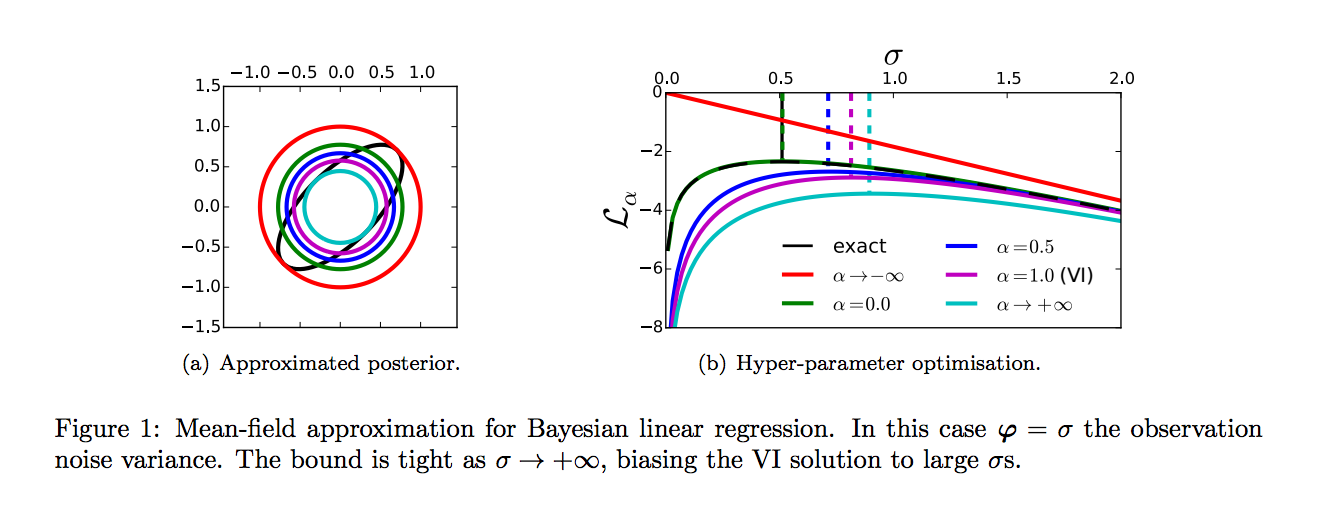
This is all well but variational inference has some drawbacks, as illustrated in Figure 1 of the paper.
- learning: the VI bound is not always very tight, and maximising the bound instead of the actual likelihood can lead to bias. Typically it biases us toward simpler models where the simple approximate $q$ has an easier job approximating the real posterior.
- inference: the $ KL[🦄|🐉]$ does not always lead to best results, it tends to favour approximate distributions $q$ that underestimate the entropy of the true posterior.
So here is the meat. The paper suggests generalising the variational bound by replacing the KL divergence with a general class of divergences called Rényi or $\alpha$-divergences.
$$
D_{\alpha}[p|q] = \frac{1}{\alpha-1}\log \int p(x)^{\alpha}q(x)^{1-\alpha}dx
$$
This general class of divergences contains as special case $KL[p|q]$ when $\alpha=1$, and a bunch of other interesting divergences. The cool thing is, we can use it to construct an alternative lower bound:
\begin{align}
\mathcal{L}_{\alpha}(x,\theta,\psi) &= \log p(x) - D_{\alpha}[p(z\vert x;\theta)|q(z\vert x;\psi)] \\
&= \frac{1}{1-\alpha} \log \mathbb{E}_{q} \left[ \left(\frac{p(x,z;\theta)}{q(z\vert x;\psi)}\right)^{1-\alpha}\right]
\end{align}
So again, 🦄 helps us defeat 🐉 and 🦂 by turning them into a cute 🐨:
$$
\log({\Large 🦂}) - \operatorname{D_\alpha}[{\Large 🦄}|{\Large 🐉}] = \frac{1}{1-\alpha} \log \mathbb{E}_{{\Large 🦄}} \left[ \left(\frac{{\Large 🐨}}{{\Large 🦄}}\right)^{1 - \alpha} \right]
$$
Awesome. So now instead of one lower bound, we have a whole family of bounds parametrised by $\alpha$. In fact, the bound becomes exact for $\alpha$ approaching $0$, this special case results in the same algorithm as Importance Weighted Autoencoders (IWAE). Cool.
Moreover, the bound becomes an upper bound for negative $\alpha$. So you can use a pair of lower and upper bounds to get a sandwitch estimate of the log-likelihood. All very nice.
Figure 1 of the paper shows how the Rényi-divergence-based bound addresses the concerns we had about the variational bound: For inference our variational posterior captures more variance, and for learning using lower $\alpha$ can reduce the bias of our parameter estimate.
🤔 This is too good to be true, what's the catch?
The catch is that the Monte Carlo estimate to deal with the $\mathbb{E}_{q}$ bit now produces a biased estimate because the averaging takes place inside the $\log$ (see Jensen's inequality) whereas before it was outside. This means that the Monte Carlo estimate will typically underestimate the bound. Ouch. So although we have a tighter bound, via Monte Carlo we loose some of the benefits.
So this means that we can choose between:
- a bound for which we have an unbiased estimator
- a family of tighter bounds for which we have a bias towards underestimating
Summary
This paper is definitely worth a read, and has a lot more to it than just deriving the bound. It proposes a practical algorithm VR-max, which uses $\alpha \rightarrow \infty$ and a smaller number of Monte Carlo samples. This method perfroms similarly to IWAE but requires fewer backpropagation iterations.