mixup: Data-Dependent Data Augmentation

By popular demand, here is my post on mixup, a new data augmentation scheme that was shown to improve generalization and stabilize GAN performance.

• H Zhang, M Cisse, YN Dauphin and D Lopez-Paz (2017) mixup: Beyond Empirical Risk Minimization

I have to say I have not seen this paper before people on twitter suggested I should write a post about this - which was yesterday. So these are all very fresh thoughts, warranty not included.

Summary of this post

• I start by introducing mixup, and immediately reformulate it in such a way that does not involve convex combinations of labels anymore, making it more comparable to traditional data augmentation. This reformulation works as long as we use binary or multinomial cross-entropy loss.
• This formulation immediately opens the door for using mixup in a semi-supervised fashion, and will help us later when thinking about its generalization properties.
• I talk about a way to understand generalization of mixup in the context of binary classification, and express the ideal test error in a form that can be evaluated in closed form for classification.
• I argue that the reason this works well for GANs is similar to why instance noise works.

Mixup

Let's jump right in the middle, here is how the mixup training loss is defined:

$$
\mathcal{L}(\theta) = \mathbb{E}_{x_1,y_1\sim p_{train}} \mathbb{E}_{x_2,y_2\sim p_{train}} \mathbb{E}_{\lambda\sim\beta(0.1)} \ell(\lambda x_1 + (1 - \lambda) x_2, \lambda y_1 + (1 - \lambda) y_2)
$$

Very simply, we take pairs of datapoints $(x_1, y_1)$ and $(x_2, y_2)$, then choose a random mixing proportion $\lambda$ from a Beta distribution, and create an artificial training example $(\lambda x_1 + (1 - \lambda) x_2, \lambda y_1 + (1 - \lambda) y_2)$. We train the network by minimizing the loss on mixed-up datapoints like this. This is all.

One intuition behind this is that by linearly interpolating between datapoints, we incentivize the network to act smoothly and kind of interpolate nicely between datapoints - without sharp transitions.

Reformulation

Now, let's assume the loss $\ell$ is linear in it's second argument, such that

$$
\ell(x, p y_1 + (1 - p) y_2) = p \ell(x, y_1) + (1 - p) \ell(x, y_2)
$$

This is the case in classification, where the loss is the binary cross entropy $\ell(x,y) = - y log p(x;\theta) - (1 - y) log (1 - p(x;\theta))$. It also works the same way for one-hot-encoded categorical labels.

In these cases, we can rewrite the mixup objective as

\begin{align}
&\mathbb{E}_{x_1,y_1\sim p_\mathcal{D}} \mathbb{E}_{x_2,y_2\sim p_\mathcal{D}} \mathbb{E}_{\lambda\sim\beta(\alpha, \alpha)} \ell(\lambda x_1 + (1 - \lambda) x_2, \lambda y_1 + (1 - \lambda) y_2) =\\
&\mathbb{E}_{x_1,y_1\sim p_\mathcal{D}} \mathbb{E}_{x_2,y_2\sim p_\mathcal{D}} \mathbb{E}_{\lambda\sim\beta(\alpha, \alpha)} \lambda \ell(\lambda x_1 + (1 - \lambda) x_2, y_1) + (1 - \lambda) \ell(\lambda x_1 + (1 - \lambda) x_2, y_2)=\\
&\mathbb{E}_{x_1,y_1\sim p_\mathcal{D}} \mathbb{E}_{x_2,y_2\sim p_\mathcal{D}}
\mathbb{E}_{\lambda\sim\beta(\alpha, \alpha)}
\mathbb{E}_{z \sim Ber(\lambda)} z \ell(\lambda x_1 + (1 - \lambda) x_2, y_1) + (1 - z) \ell(\lambda x_1 + (1 - \lambda) x_2, y_2)=\\
&\mathbb{E}_{x_1,y_1\sim p_\mathcal{D}} \mathbb{E}_{x_2,y_2\sim p_\mathcal{D}}
\mathbb{E}_{z \sim Ber(0.5)}
\mathbb{E}_{\lambda \sim \beta(\alpha + 1 - z, \alpha + z)} z \ell(\lambda x_1 + (1 - \lambda) x_2, y_1) + (1 - z) \ell(\lambda x_1 + (1 - \lambda) x_2, y_2)=\\
&\frac{1}{2}\mathbb{E}_{x_1,y_1\sim p_\mathcal{D}} \mathbb{E}_{x_2,y_2\sim p_\mathcal{D}}
\mathbb{E}_{\lambda \sim \beta(\alpha, \alpha + 1)} \ell(\lambda x_1 + (1 - \lambda) x_2, y_1) +
\frac{1}{2}\mathbb{E}_{x_1,y_1\sim p_\mathcal{D}} \mathbb{E}_{x_2,y_2\sim p_\mathcal{D}}
\mathbb{E}_{\lambda \sim \beta(\alpha + 1, \alpha)} \ell(\lambda x_1 + (1 - \lambda) x_2, y_2) = \\
&\mathbb{E}_{x,y\sim p_\mathcal{D}}
\mathbb{E}_{x'\sim p_\mathcal{D}}
\mathbb{E}_{\lambda \sim \beta(\alpha, \alpha + 1)}
\ell(\lambda x + (1 - \lambda) x', y)
\end{align}

Line by line, I used the following tricks:

1. linearity of the loss, as in assumption above
2. expectation of a Bernoulli($\lambda$) variable plus linearity of expectation
3. Bayes' rule $p(z\vert \lambda)p(\lambda) = p(\lambda\vert z)p(z)$ and the fact that the Beta distribution is conjugate prior for the Bernoulli
4. expectation of a Bernoulli(0.5) plus linearity of expectation
5. symmetry of the Beta distribution in the sense that $\lambda \sim Beta(a,b)$ implies $1-\lambda \sim Beta(b,a)$, plus changing variable names in the expectation so the two terms become the same

So, here is what we are left with:

$$
\mathcal{L}(\theta) = \mathbb{E}_{(x,y)\sim p_\mathcal{D}}
\mathbb{E}_{\lambda \sim \beta(\alpha, \alpha + 1)}
\mathbb{E}_{(x')\sim p_\mathcal{D}}
\ell(\lambda x + (1 - \lambda) x', y)
$$

I think this formulation is much nicer, because:

• you no longer have blending of labels, which to me was weirdest thing to begin with. This is a lot like the usual data augmentation, which only manipulates the input $x$, but keeps the label $y$ the same. The only thing that changes compared to data augmentation is that the vicinal distribution (augmentation distribution) applied to $x$ is dependent on $p_{train}(x)$, the distribution of inputs.
• we no longer use the joint distribution $p_\mathcal{D}(x,y)$, but only $p_\mathcal{D}(x)$ to define the vicinal distribution. This means that, technically, this form can be used in a semi-supervised setting, as follows:

$$
\mathcal{L}(\theta) =
\mathbb{E}_{x,y\sim p_\mathcal{\text{labelled}}}
\mathbb{E}_{\lambda \sim \beta(\alpha, \alpha + 1)}
\mathbb{E}_{x'\sim p_\mathcal{\text{unlabelled}}}
\ell(\lambda x + (1 - \lambda) x', y)
$$

Pytorch code

Here's how you'd modify the pytorch code from the paper to make this work (I draw different lambdas per datapoint in the minibatch, they draw one lambda per minibatch, not sure which one works better):

for (x1, y1), (x2, _) in zip(loader1, loader2):
    lam = numpy.random.beta(alpha+1, alpha, batchsize)
    x = Variable(lam * x1 + (1. - lam) * x2)
    y = Variable(y1)
    optimizer.zero_grad()
    loss(net(x), y).backward()
    optimizer.step()

Only three changes:

• you ignore the labels y2 from the second minibatch - hence the _
• lambda is now drawn from an asymmetric $Beta(\alpha,\alpha+1)$ (note numpy orders arguments of beta differently).
• you just use the label from the first minibatch - no blending there

This should do roughly the same thing.

Let's visualize this

Let's look at what the this data-dependent augmentation looks like for a single datapoint on the two-moons dataset:

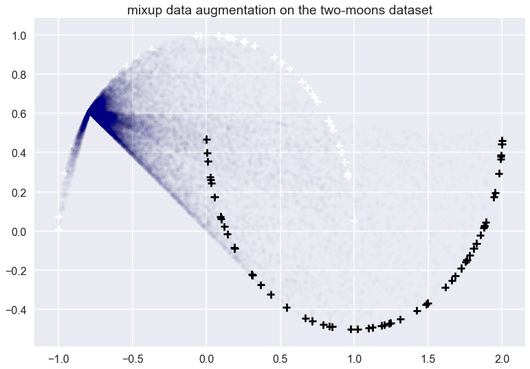
The white and black crosses are positive and negative examples respectively. The mixup data augmentation doesn't care about the labels, just the distribution of the data. I applied the mixup to the datapoint at roughly $x=(-0.7, 0.6)$. The transparent blue dots show random samples from the vicinal distribution. Each blue point was obtained by picking another training datapoint $x'$ at random, then picking a random $\lambda$ from a $Beta(0.1, 1.1)$ and then interpolating between $x$ and $x'$ accordingly. Note that $Beta(0.1, 1.1)$ is not symmetric, roughly 80% of sampled $\lambda$ will be higher than $0.9$ sowe tend to end up much closer to $x$ than $x'$. All these blue dots would be added to the training data with a 'white' label.

This is what the picture looks like when we applied data augmentation to two training examples, one positive, and one negative, and using 10k unlabelled samples (I am plotting a few of those unlabelled samples for reference):

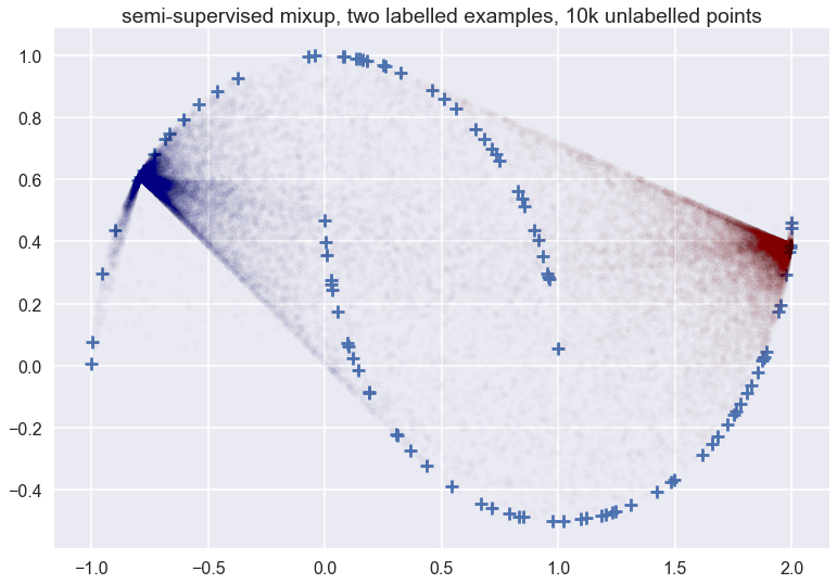
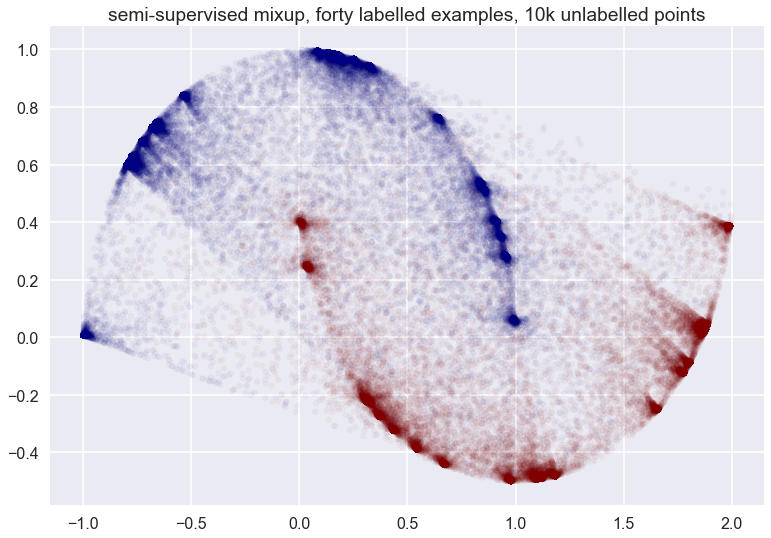
You can see that the vicinal distribution of mixup does not really follow the manifold - which one would hope a good semi-supervised data augmentation scheme would do in this particular example. It does something rather weird. Things don't look that much cleaner whe we have more labelled examples:

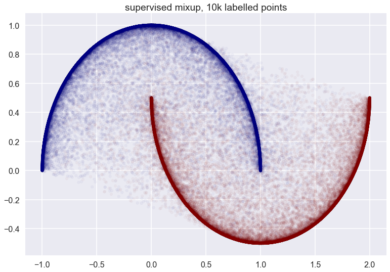
Finally, with all datapoints labelled:

Why should data augmentation generalize better?

Why should a data augmentation scheme - or vicinal risk minimization (VRM) generalize better in classification? Generalization gap is about the difference between training and validation losses which is there because the training and test distributions differ (in practice, these are both empirical distributions concentrated on a number of samples). Vicinal risk minimization (VRM) or data augmentation trains by minimizing risk on the augmented training distribution:

$$
p_{\text{aug}}(x,y) = \frac{1}{N_{train}}\sum_{x,y\in \mathcal{D}_{train}} \nu(x', y'\vert x, y),
$$

for some vicinal distribution $\nu(x', y'\vert x, y)$. This should be successful if the augmented distribution $p_{aug}$ actually ends up closer to $p_{test}$ than the original training $p_{train}$. Following the ideas of (Lacoste-Julien et al, 2011), also or section 1.3.7 of my PhD thesis, we can even find the divergence measure we should use to measure the difference between these distributions, based on Bayes decision theory. If we use the binary cross-entropy both for training and testing, the Bayes optimal decision function on the augmented data will be (assuming perfectly balanced classes):

$$
q_{aug}(x) = \frac{p_{aug}(x\vert 1)}{p_{aug}(x\vert 1) + p_{aug}(x\vert 0)}
$$

When mixup mixes up the empirical distribution of the two classes, it turns them into continuous distributions with perfectly overlapping support. Therefore, the Bayes optimal decision function is more or less unique, so we should be able to find $q_{aug}(x)$, or something very close to it quite consistently during training.

The loss of this optimal training classifier $q_{aug}(x)$ on the test data is as follows:

\begin{align}
\mathcal{L}_{test}(q_{aug}) &= \mathbb{E}_{y\sim p_{test}} \mathbb{E}_{x\sim p_{test}(x\vert y)} - \log(p_{aug}(x\vert y)) + \mathbb{E}_{x \sim p_{test}} \log(p_{aug}(x)) \\
&= \mathbb{E}_{y\sim p_{test}} \operatorname{KL}[p_{test}(x\vert y) | p_{aug}(x\vert y)] - \operatorname{KL}[p_{test}(x) | p_{aug}(x)]
\end{align}

Interestingly, if we use $p_{test}(x)$ in the mixup, we an actually evaluate these quantities exactly, which gives us a lower bound on the training error.

So, let's answer the question: why might data augmentation generalize better:

1. because the training loss becomes better defined such that the Bayes-optimal solution is unique and easier to find consistently. In the case of mixup this happens because to the fact that the class-conditional distributions end up having fully overlapping support.
2. because data augmentation turns the training distribution into a distribution that is closer to the test distribution. The ideal generalization gap can be seen as Bregman divergence between $p_{test}$ and $p_{aug}$, up to a constant. In the case of mixup, we can actually calculate this divergence if we use $p_{train}(x)$ in the vicinal distribution.

Why should it work well for GANs?

I suspect reason number 1 above also explains why mixup works well for training GANs. One of the issues with the usual GAN setup is that the training and synthetic distributions have widely different support, and are often concentrated to lower-dimensional manifolds.

Instance noise was initially introduced to alleviate this problem by making the support of the two distributions overlap. See also (Arjovsky and Buttou, 2017). Mixup achieves the same thing, and I would imagine it does so even better in practice.

Why should it work well against adversarial examples?

Resilience to adversarial examples is somewhat related to, but crucially different from generalization. Firstly, the test data in the adversarial setting $p_{test}$ is generated specifically to fool our classification function - it's no longer independent of the training set or the training algorithm. Secondly, and crucially, adversarial examples are created on the basis of the gradient of the decision function. However, the training loss only depends on values of the decision function at certain training points. For a decision function to achieve minimal training loss, it doesn't even have to be differentiable, or continuous. In fact, we could even implement it as a look-up-table, which would be memorization. So adversarial examples are created by a property of the decision function that the empirical loss is perfectly insensitive to.

The way mixups addresses this is twofold:

1. due to the vicinal distribution, the training loss function suddenly starts to care about a local neighbourhood of the decision function around a training datapoint - and the behaviour in that local neighbourhood will depend on the gradients.
2. It is evident from the figures above that mixup tends to produce data augmentations to cover the likely location of where adversarial examples might end up.

Summary

note that I have updated the summary as I reevaluated my conclusions.

Mixup is an interesting technique, but I don't believe it's the final version that we will see in the wild. My initial instinct was to somehow combine this idea with nearest-neighbour-like things which tend to work quite well for manifold-like data. For example: restrict mixup only between nearest neighbours, or make $\alpha$ depend on distance. After another day of thinking, I'm not so sure that's a great idea generally. Although incorporating nearest-neighbour to mixup would probably look very good on the 2D two-moons toy example, real data doesn't look like that. More importantly, real data people want to apply this to is high dimensional. Nearest neighbour methods in pixel space probably wouldn't work quite as well as they do on the nice 2D manifold for the same reason Gaussian noise doesn't work very well for high-D problems.