
How powerful are Graph Convolutions? (review of Kipf & Welling, 2016)
This post is about a paper that has just come out recently on practical generalizations of convolutional layers to graphs:
- Thomas N. Kipf and Max Welling (2016) Semi-Supervised Classification with Graph Convolutional Networks
Along the way I found this earlier, related paper:
- Defferrard, Bresson and Vandergheynst (NIPS 2016) Convolutional Neural Networks on Graphs with Fast Localized Spectral Filtering
This post is mainly a review of (Kipf and Welling, 2016). The paper is nice to read, and while I like the general idea, I feel like the approximations made in the paper are too limiting and severely hurt the generality of the models we can build. This post explains why. Since writing this, Thomas also wrote a blog post addressing some of my comments, which I highly recommend.
Summary of this post
- Graph convolutions are generalisation of convolutions, and easiest to define in spectral domain
- General Fourier transform scales poorly with size of data so we need relaxations
- (Kipf and Welling) use first order approximation in Fourier-domain to obtain an efficient linear-time graph-CNNs
- I illustrate here what this first-order approximation amounts to on a 2D lattice one would normally use for image processing, where actual spatial convolutions are easy to compute
- in this application the modelling power of the proposed graph convolutional networks is severely impoverished, due to the first-order and other approximations made.
The general graph-based learning problem
The graph learning problem is formulated as follows:
- we are given a set of nodes, each with some observed numeric attributes $x_i$.
- For each node we'd like to predict an output or label $y_i$. We observe these labels for some, but not all, of the nodes.
- We are also given a set of weighted edges, summarised by an adjacency matrix $A$. The main assumption is that when predicting the output $y_i$ for node $i$, the attributes and connectivity of nearby nodes provide useful side information or additional context.
Kipf & Welling use graph convolutional neural networks to solve this problem. A good way to imagine what's happening is to consider a neural network that receives as input features $x_j$ from all nodes $j$ in the local neighbourhood around a node $i$, and outputs an estimate of the associated label $y_i$. The information from the local neighbourhood gets combined over the layers via a concept of graph convolutions.
The deeper the network, the larger the local neighbourhood - you can think of it as the generalisation of the receptive field of a neuron in a normal CNN. This network is applied convolutionally across the entire graph, always receiving features from the relevant neighbourhood around each node.
How are convolutions on a graph defined?
Usually, when we talk about convolutions in machine learning we consider time series, 2D images, occasionally 3D tensors. You can understand these as special cases of the graph learning problem, where the graph is a regular line, 2D square or 3D cube lattice with regular connectivity between neighbouring pixels or tensor entries.
These are all examples or regular graphs where all nodes have the same neighbourhood connectivity patterns. It's not immediately obvious/intuitive how to generalise the concept of convolutions to arbitrary graphs that can have nodes with very different local connectivity patterns or different degrees.
To generalise the concept, we need to adopt a spectral view on convolutions, and consider what convolutions are in Fourier-domain: simple pointwise multiplication of the Fourier-transform of a signal. Fourier-transforms do generalise to graphs, therefore we can define a general concept of graph convolutions as pointwise multiplication of the spectra of signals in Fourier-domain.
This, however, is a very impractical view: computing the spectrum of signal over general graphs involves matrix diagonalisation, which generally has cubic complexity in the number of nodes. Computing exact convolutions over graphs is thus computationally intensive.
Approximate graph convolutions
One way to make graph convolutions work is by limiting the convolution kernels under consideration. For example, if the conv. kernel can be expressed or approximated using Chebyshev polynomials of eigenvalues in spectral domain, computing the convolution becomes easier. Like Taylor-expansion, this Chebyshev approximation can be made arbitrarily accurate by making $k$ higher. This is the approach proposed earlier this year:
- Defferrard, Bresson and Vandergheynst (NIPS 2016) Convolutional Neural Networks on Graphs with Fast Localized Spectral Filtering
Kipf & Welling also use use this trick, but go even further and only use a $1^{\text{st}}$ order approximation. In the Fourier domain, this restricts convolutions to kernels whose spectrum is an affine function of eigenvalues.
This makes computations pretty fast and easy, and the authors show competitive results on a bunch of graph-learning datasets. But what is really the price we pay when we use this first order approximation? This is what I'll try to illustrate in this post.
Special case: dense prediction in computer vision
I think it's intuitive to consider the behaviour of the algorithm in a well-studied special case: dense prediction in image processing, such as binary segmentation. Here
- the node values $x_i$ are RGB, YUV or for simplicity just grayscale pixel intensities
- the output per node $y_i$ can be a binary or discrete label in semantic segmentation or pixel intensities in image denoising or stylization
- the graph is defined over a regular 2D square lattice of 8-connected pixels as shown below
- let's assume the graph has 4-way rotational symmetry, so all horizontal and vertical edges share the same weight $\alpha$ and all diagonal edges have weight $\beta$.
- let's further assume the lattice is infinitely large just so we don't have to worry about what happens at borders
In this application, the graph convolutional network model from Kipf & Welling equates to a vanilla multilayer convolutional neural network, with only convolutional layers, no pooling or anything else. So far, this is good news, as these CNNs can actually solve a lot of dense prediction problems just fine, even though additional operations such as pooling-deconvolution generally can help a lot, such as in hourglass-shaped models.
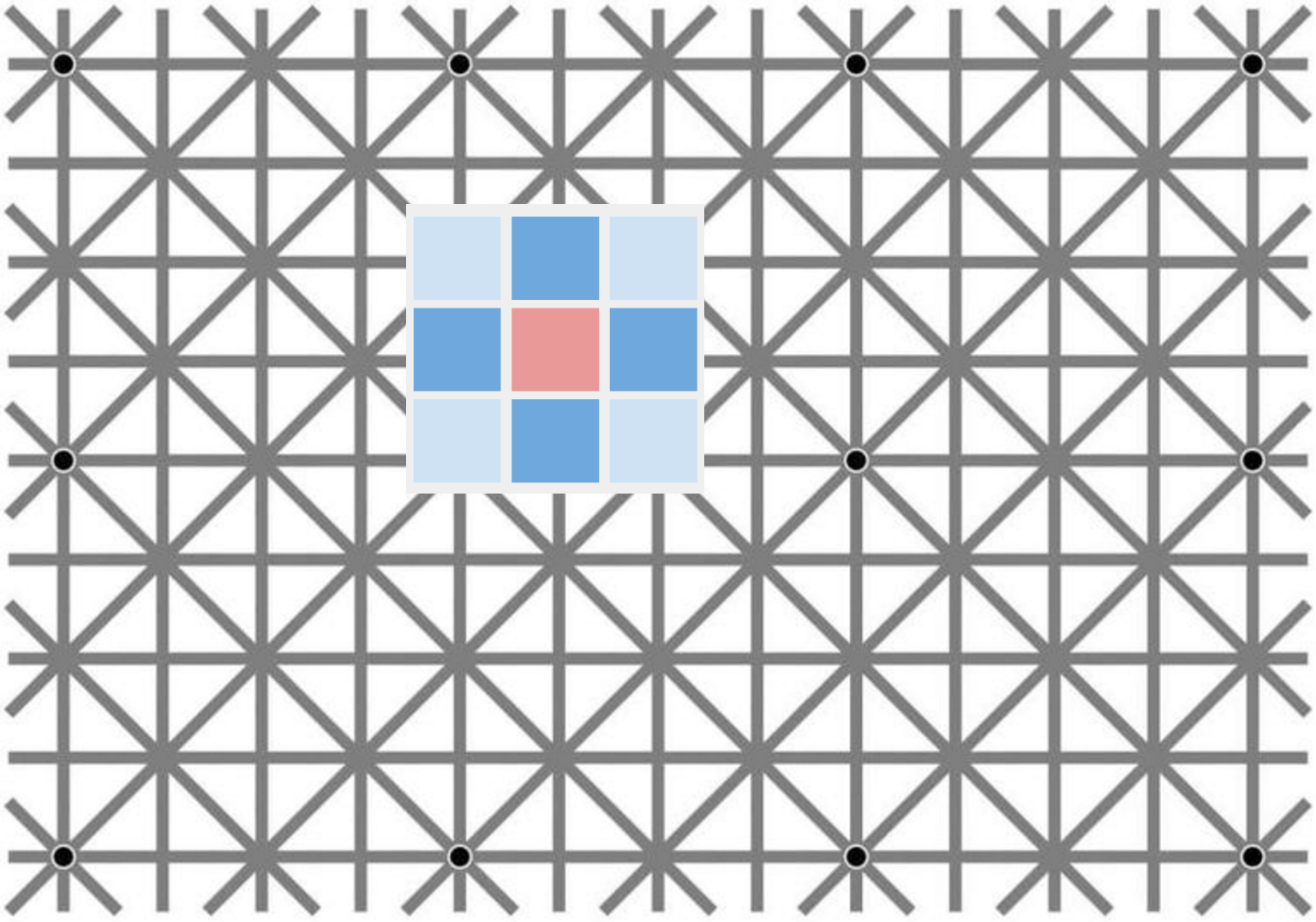
However, the approximation employed in the Kipf & Welling model severely restricts the convolution filters available to us. At all levels in this network, the filters are limited to $3\times 3$ in size (which in itself is still OK) and are also essentially fixed to be the same kernel across all layers and all units in entire network, up to a constant multiplier! 😱
If we use the two-parameter approximation in Eqn. 6, the kernel basically becomes a center-surround pattern like the one pictured above, mathematically, something like this:
$$
\left[\matrix{
\theta_1 c_1&&\theta_1 c_2&&\theta_1 c_1\\
\theta_1 c_2&& \theta_0 + \theta_1 c_3&& \theta_1 c_2\\
\theta_1 c_1&&\theta_1 c_2&&\theta_1 c_1\\
}\right],
$$
where $c_1$, $c_2$ and $c_3$ are fixed constants that depend on the graph weight parameters $\alpha$ and $\beta$ only. The only trainable parameters are $\theta_0$ and $\theta_1$, and in the final version the authors even further fix $\theta_0 = -\theta_1$ so that the kernel only has a single scalar trainable parameter - essentially a scalar multiplier. Details on how $c_1$, $c_2$ and $c_3$ are computed aside, this model is in fact very, very limited.
Imagine trying to solve something like image segmentation with a CNN where only a particular, fixed centre-surround receptive field is allowed - pretty much impossible. I don't think it's even possible to learn edge-detectors, or Gabor-like filters, or anything sophisticated, even with a multilayer network and lots of nonlinearities.
Summary
I'm not saying that the model proposed by Kipf & Welling cannot work well in some practical situations, indeed they show that it achieves competitive results in a number of benchmark problems. Also, their approach applies generally to graphs, of which regular 2D-3D lattices are a very unlikely special case, so it is to be expected that models developed for a more general problem will have less power.
However, the 2D lattice example highlights, the generality and flexibility of this model is, at least in its present form, seriously lower than the CNNs we are used to in image processing. CNNs are a kind of super-weapon, a dependable workhorse when you need to solve pretty much any kind of problem. When you read graph convolutional networks it sounds like we now have a similarly powerful megaweapon to deal with graphs. Unfortunately, this may not be the case yet, but these papers certainly point in that very interesting direction.
From the perspective of generality, the more general treatment of Defferrard et al (2016) looks more promising, even with the added computational burden of including higher order Chebyshev polynomials in the approximation.