Evolution Strategies: Almost Embarrassingly Parallel Optimization

I watched Ilya Sutskever's talk on their new evolutionary strategies paper. Here's the paper:

• Salimans et al (2017) Evolution Strategies as a Scalable Alternative to Reinforcement Learning

The reason this paper is fascinating is that they use a relatively dumb, simple stochastic method of optimisation that shouldn't really work well in practice, and show that it is actually competitive with SGD/back-propagation-based methods in RL. This is mainly due to the fact that it parallelizes so naturally. In this respect it's an eye-opening paper.

In this note I explain the rather basic math behind the technique, and talk a bit about a few random ideas that may further improve the efficiency of the method:

• second order derivatives
• importance sampling for variance reduction
• reusing samples from previous steps
• Bayesian optimisation

Caveat: I am pretty sure there is vast literature on evolution strategies and related methods that I am simply not familiar with. This post is a collection of my first ideas I had after my first encounter with this technique. It is highly likely, almost certain, that many of the things I talk about here have been done before - sorry if I miss references.

If you're interested in, also check out David Barber's post on variational optimisation and its connections to ES.

What is ES?

Evolution strategies (ES) is can be best described as a gradient descent method which uses gradients estimated from stochastic perturbations around the current parameter value. While the authors did comparisons in the context of RL, and there are many RL-specific advantages, here I'm focussing on ES as a general black-box optimisation method.

The main observation is this: if $f$ is a differentiable function with respect to $\theta$, it's gradients can be approximated as follows:

$$
\frac{\partial}{\partial \theta}f(\theta) \approx \frac{1}{\sigma^2}\mathbb{E}_{\epsilon \sim \mathcal{N}(0,\sigma^2)} \epsilon f(\theta + \epsilon)
$$

It's actually very easy to see why. Let's approximate $f$ locally as a second-order Taylor expansion (I'm going to write everything as for one dimensional $\theta$ to simplify notation, but it works out analogously in the multivariate case as well):

$$
f(\theta+\epsilon) \approx f(\theta) + f'(\theta)\epsilon + \frac{f''(\theta)\epsilon^2}{2}
$$

Substituting this back to the expectation before we have that:

\begin{align}
\mathbb{E}_{\epsilon \sim \mathcal{N}(0,\sigma^2)} \epsilon f(\theta + \epsilon) &= \mathbb{E}_{\epsilon \sim \mathcal{N}(0,\sigma^2)} \left[ f(\theta)\epsilon + f'(\theta)\epsilon^2 + \frac{f''(\theta)\epsilon^3}{2} \right] \\
&= f'(\theta) \sigma^2,
\end{align}

using the fact that the $p^{th}$ central moment of a Gaussian is always $0$ for odd $p$.

This is it. In each step, ES perturbs the current parameter value by additive Gaussian noise, evaluates the function at the perturbed values, finally combines these function values into a gradient estimate and takes a step in that direction.

Here is a figure taken from OpenAI's blog post visually illustrating how the method works for optimising a 2D function:

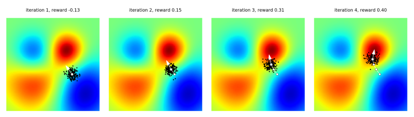
When $\theta$ is high dimensional, this approximation can have very high variance, so common sense dictates you shouldn't use this in practice, especially when you can actually calculate gradients via back-propagation. The ES paper, however, debunked common sense.

ES can be a very competitive method in scenarios when:

• you have a very large number of nodes to distribute computations to
• your parameter space is huge so sending parameter values between nodes would be expensive
• you are dealing with a non-differentiable objectives where SGD doesn't quite work or needs approximations.

Almost embarrassingly parallel

Distributed versions of SGD exist, but they almost always need to communicate parameter updates between nodes, or to a central parameter server. When your parameter-space is huge, sending a high-dimensional $\theta$ over the network quicklih becomes the most time consuming thing you do, slowing everything down a bit.

Distributed ES use a smart observation: Each worker calculates $f_i = f(\theta + \epsilon_i)$ for its own $\epsilon_i$. To estimate the gradient, one needs all the $\epsilon_i$s and all the computed $f_i$ values. Communicating $f_i$s is cheap as they are scalars, communicating $\epsilon_i$s are just as expensive as communicating $\theta$. However, since $\epsilon_i$ are pseudorandom numbers you don't need to communicate these assuming workers know each others' random seed. The workers can simulate other workers' random number generators locally.

This makes distributed ES almost embarrassingly parallel, where only single scalars need to be communicated in each update cycle. This time saving, combined with the fact that we don't do back-prop (which is typically about twice as time consuming than the forward pass), makes ES super fast compared to SGD. So even though your gradient estimates are noisy, you can take a lot more noisy gradient steps in the same timeframe. Ironically, This has a similar effect to reducing the batchsize in SGD: your gradients get noisier, but you update more frequently.

Non-differentiability

SGD deals with objective functions which are of the following form - broadly speaking:

$$
f(\theta) = \mathbb{E}_{x} f(\theta; x)
$$

SGD requires that individual $f(\theta; x)$ are all differentiable w.r.t. $\theta$ for all values of $x$. In this case you can just swap the expectation with the differentiation as follows:

$$
\frac{\partial}{\partial \theta}f(\theta) = \mathbb{E}_{x} \frac{\partial}{\partial \theta}f(\theta; x)
$$

However, in many applications $f(\theta; x)$ is not actually differentiable. Examples include:

• POMDPs/RL with discrete action or state space
• variational autoencoders with discrete latent variables (Jang et al, 2016)
• GANs with discrete generators (Hjelm et al, 2017)

ES still works in these scenarios, because you can simply swap expectations with respect to $x$ and $\epsilon$ (unlike swapping the expectation with the differentiation).

\begin{align}
\mathbb{E}_\epsilon \epsilon f(\theta + \epsilon) &= \mathbb{E}_\epsilon \epsilon \mathbb{E}_{x} f(\theta + \epsilon; x) \\
&= \mathbb{E}_{x} \mathbb{E}_\epsilon \epsilon f(\theta + \epsilon; x)
\end{align}

This is why ES is so powerful in RL: it can solve RL problems in a way that is not possible with explicit stochastic gradient descent, because the reward in individual episodes is not differentiable w.r.t. parameters of the policy.

Second order ES

ES is in fact a special case of SGD, rather than an alternative. The most general formulation of SGD only really requires an unbiased estimate of the gradients (unbiased = noisy but correct on average). In the usual minibatch-backprop SGD the unbiased but noisy estimates come from subsampling of i.i.d. data. In ES, the gradient estimates may be ever so slightly biased (due to the approximation of $f$ as 2nd order Taylor expansion), but for all practical purposes you can think of it as unbiased. The main difference then is the source of randomness in the gradient estimates: in backprop-SGD it's data subsampling (minibatches), in ES it's random perturbations in addition to data subsampling. As a result, all the tricks you could apply to backprop SGD you can still apply to ES and expect success. The authors show that batchnorm, Adam, etc. still work, for example.

Is there anything ES can do that normal backprop-SGD cannot? Well, for one, you can compute direct estimates of second order gradients with minimal overhead using exactly the same $(\epsilon_i, f_i)$ pairs you used to estimate gradients:

\begin{align}
\mathbb{E}_\epsilon \left(\frac{\epsilon^2}{\sigma^2} - 1\right) f(\theta+\epsilon) &\approx
\frac{1}{\sigma^2}\mathbb{E}_{\epsilon} \left[ f(\theta)\epsilon^2 + f'(\theta)\epsilon^3 + \frac{f''(\theta)\epsilon^4}{2} \right] -
\mathbb{E}_{\epsilon} \left[ f(\theta) + f'(\theta)\epsilon + \frac{f''(\theta)\epsilon^2}{2} \right]\\
&= \frac{1}{\sigma^2}\left(\sigma^2 f(\theta) + 3 \sigma^4 f''(\theta)\right) - \left(f(\theta) + \frac{\sigma^2 f''(\theta)}{2}\right)\\
&= \frac{\sigma^2 5}{2} f''(\theta)
\end{align}

Of course this estimate may be biased and outrageously high variance as well. So, if your outer SGD algorithm allows for preconditioning with second order derivative information, you may be able to use these estimates that come out of the data you already computed for free. Some commenters mentioned that the authors already use Adam and batchnorm, and Adam and batchnorm already are approximating second order behaviour, so whether the additional noisy estimate of the Hessian can add to that remains an open question.

Importance Sampling

The variance of the estimator may be significantly reduced using importance sampling. Instead of sampling $\epsilon$ from an isotropic Gaussian, one could sample it from a different proposal distribution $q$, and then correct for the mismatch between $q$ and the Gaussian by introducing importance weights:

$$
\mathbb{E}_{\epsilon\sim \mathcal{N}}\left[ \epsilon f(\theta + \epsilon)\right[ = \mathbb{E}_{\epsilon \sim q} \left[\epsilon \frac{\mathcal{N}(\epsilon)}{q(\epsilon)}f(\theta + \epsilon)\right]
$$

As long as the workers know what the proposal distribution $q$ is, and know each others' random seed, the algorithm is still trivially parallelisable.

How can we choose a proposal distribution?

Well, one could do some sort of momentum-based proposal. Instead of drawing $\epsilon$ from a $0$-mean Gaussian, one could sample from a Gaussian with mean $\mu$ where $\mu$ is some kind of momentum of the gradient descent, like the exponential weighted average of previous gradient estimates.

Alternatively, one could use importance sampling as a way to reuse calculations from previous timesteps. In the vanilla version of ES, once you calculated the gradient estimate, you discard all the $f_i$ values. But if the parameters only move a little bit, these values might still carry a lot of information. So, they can be used to contribute to our estimate of the gradient around the new parameter $\theta$:

$$
f'(\theta) \approx \frac{1}{I} \sum_i f(\theta^{old} + \epsilon^{old}_i) \left(\epsilon^{old}_i + \theta^{old} - \theta\right) \frac{\mathcal{N}\left(\epsilon^{old}_i + \theta^{old} - \theta; 0, \sigma^2\right)}{\mathcal{N}\left(\epsilon^{old}_i; 0, \sigma^2\right)}
$$

distributed Bayesian optimisation

Another thought is this: once you have calculated the function value at a bunch of perturbed locations, can you do something smarter with those $(\epsilon_i, f_i)$ pairs than using a second order Taylor approximation? In particular, imagine you could use some simple machine learning to perform local regression of the objective function, and jump right into where you expect the most significant gain. This only works of course, if the regression and subsequent optimisation steps can be done very cheaply and quickly, otherwise you're taking time away from other things like calculating derivatives, or evaluating the function at more points. But there may be a sweet-spot where the workers know each other's random seed idea can be applied more generally in a Bayesian optimisation setting.

Summary

This paper may be controversial, some think it's overhyped. I don't think it is, I think there's something in there, and this may be the beginning of a new line of research (well, within deep learning, much of these have probably been done by optimisation people before). I personally find the terminology 'Evolution Strategies' quite unfortunate (it's not the authors of this paper who came up with the nname). I think it's going to be much more fruitful for machine learning to think about this method from the perspective of stochastic gradient estimates than as a special case of evolutionary algorithms as the name implies.

Previously, very good things have come out of researchers questioning fundamental assumptions about our methods: If you think about it, replacing smooth sigmoid activations with non-differentiable rectified linear units sounds like a pretty bad idea - until you actually realise they work. Dropout may sound like something to be avoided, until you realise why it works. Stochastic gradient descent was born out of necessity: you couldn't fit more than a certain amount of data on a GPU, and it was impractical to loop over the entire dataset for each gradient update. The variance of gradient estimates was initially seen as a bad thing. But it turns out, the noise introduced by small batchsizes can actually be beneficial in itself - and even if you could do non-stochastic GD, SGD often works better.

So ES may well be one of these things. Salimans et al questioned a fundamental thing that everybody takes for granted: that neural networks are optimised via SGD using backpropagation. Well, maybe not always.