Evolution Strategies, Variational Optimisation and Natural ES
In my last post I conveyed my enthusiasm about evolution strategies (ES), and particularly the highly scalable distributed version. I have to admit, this was the first time I had come across this particular formulation, and unexpectedly, people were quick to point out a whole body of research that I probably should have read or known about.
Here, I want to highlight two such papers:
- Staines and Barber (2013) Optimization by Variational Bounding ESANN
- Wierstra et al (2014) Natural Evolution Strategies JMLR
And I also highly recommend David's blog post. This post is just a summary of what I've learnt about ES, a bit of an addendum to last week's post. Thanks to David Barber, Olivier Grisel and Nando de Freitas for their comments and pointers.
The upper bound view
In optimisation we seek the global minimum of a function. The value of the minimum can be upper bounded by minimum over average function values as follows:
$$
\min_x f(x) \leq \min_\theta \mathbb{E}_{x\sim p(x\vert \theta)} [f(x)] = \min_\theta J(\theta,f)
$$
This is pretty easy to prove: the average (convex combination) of a set of numbers can never be lower than the lowest number in that set.
So, instead of optimising $f(x)$ w.r.t. $x$, one can optimise $J(\theta,f)$ with respect to $\theta$. Staines and Barber call this Variational Optimisation (VO), a name I much prefer to evolution strategies (ES). Crucially, even if $f$ itself is non-differentiable, $J(\theta)$ might be. This means it makes sense to run gradient descent on it. The gradient $\nabla_\theta J(\theta,f)$ itself can be conveniently expressed as:
\begin{align}
\frac{\partial}{\partial \theta} \mathbb{E}_{x\sim p(x\vert \theta)} f(x) &= \frac{\partial}{\partial \theta} \int p(x\vert \theta) f(x) dx\\
&= \int \frac{\partial}{\partial \theta} p(x\vert \theta) f(x) dx\\
&= \int p(x \vert \theta) \frac{\partial}{\partial \theta} \log p(x\vert \theta) f(x) dx \\
&= \mathbb{E}_{x\sim p(x\vert \theta)} f(x) \frac{\partial}{\partial \theta} \log p(x\vert \theta)
\end{align}
where we used the chain rule on $\log p(x\vert \theta)$. Thus, as long as we can compute the score $\frac{\partial}{\partial \theta} \log p(x\vert \theta)$, we can construct an unbiased Monte Carlo estimate to the gradient $\nabla_\theta J(\theta)$, and run SGD on $J$.
It's easy to show that when $p$ is an isotropic Gaussian with fixed covariance, the VO gradient w.r.t. $\theta$ looks exactly like our gradient estimate in vanilla evolution strategies. But what's cool about the VO formulation is that it also provides a meaningful farmework to optimise the perturbation variance $\sigma^2$, or indeed any other parameter of the sampling distribution.
Visualising what's going on
Let's consider seeking the global minimum of a 1D function, such as the sinc:
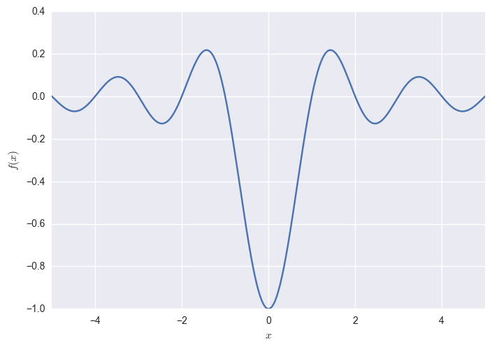
Now consider minimsing $J(\theta) = \mathbb{E}_{x\sim p(x\vert \theta)}f(x)$ using a Gaussian $p(x\vert \theta)$, whose parameters are $\theta = [\mu, \sigma]$. We have turned our 1D optimisation problem into a 2D one where the objective function looks like this:
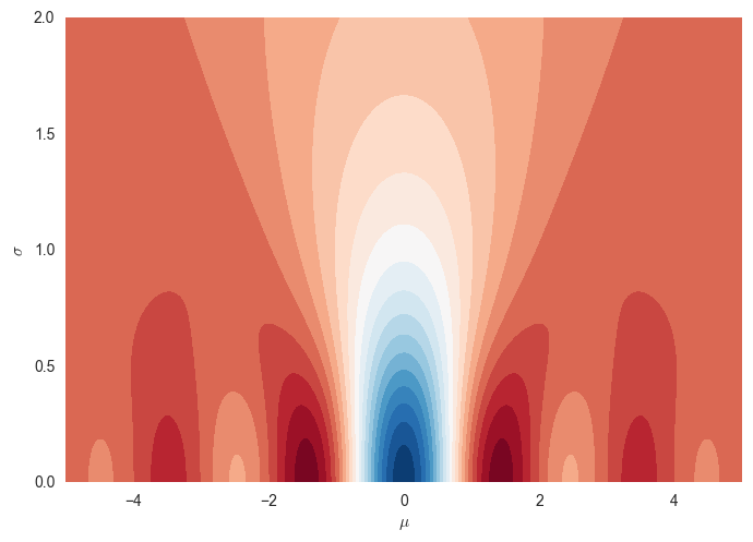
Notice a few things:
- we are now minimising $\mu$ and $\sigma$, rather than $x$
- the global minimum of this $J$ is in the blue bit at the bottom: $\mu=0$ as $\sigma\rightarrow 0$.
- if $f$ has a unique global minimum, so does $J(\mu,\sigma)$. If $f$ is convex, so is $J$.
- reaching the global minimum of $f$ via gradient descent seems tricky as it has lots of local minima, but if you start with a $\sigma$ around $1.5$, finding the global minimum of $J(\mu,\sigma)$ via gradient descent seems a lot easier.
- getting to the optimum involves going down into an increasingly narrow tunnel (the blue bit). This is a situation in which vanilla stochastic gradient descent might struggle with. You really want to use Adam, or some other smart momentum method (or natural graidents, see second part of this post) to avoid ping-ponging between the walls of this canyon.
For $\sigma\rightarrow0$ the function is the same as the original $f$, and as you increase sigma, the function starts looking more and more like a constant.
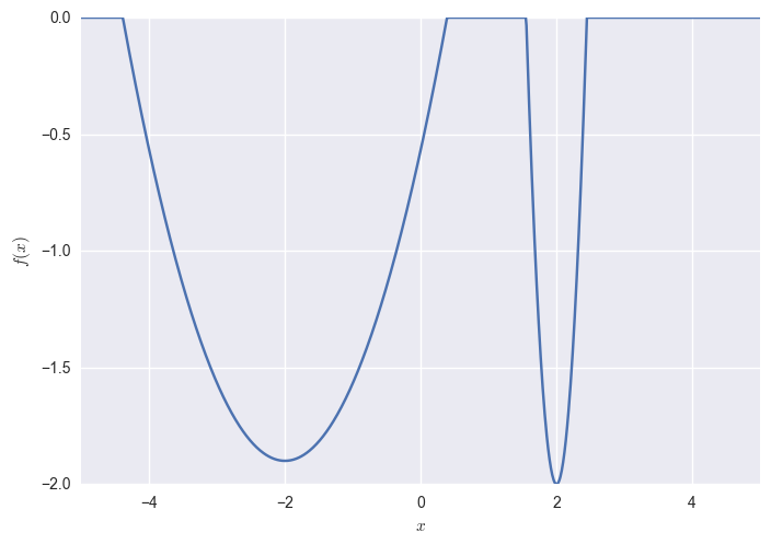
Now consider a non-differentiable function such as a quantized sinc:
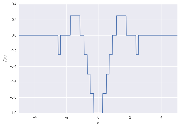
The variational bound is still differentiable (because the Gaussian pdf is differentiable) for all positive $\sigma$s, but approaches the non-differentiable $f$ as $\sigma\rightarrow 0$:
In fact, the two bounds look very similar except here you get increasingly non-differentiable behaviour as you decrease $\sigma$.
What if you don't adjust $\sigma$
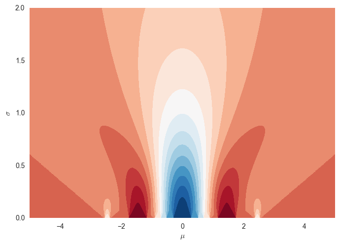
What if you keep $\sigma$ fixed in ES? What kind of problems can it cause? Consider minimsing the following function:
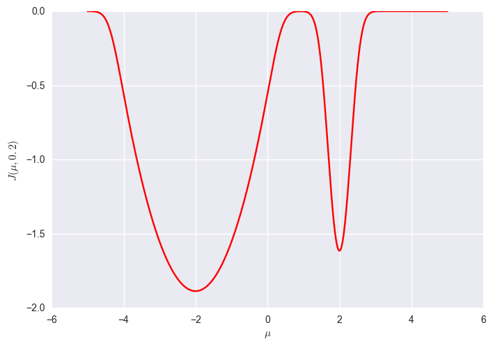
The corresponding VO objective J looks like this:
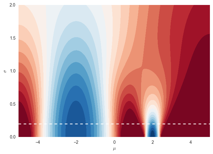
The global minimum of this objective is at $\mu=2, \sigma\rightarrow 0$. However, if you consider a fixed $\sigma=0.2$ (shown above by white dashed line), the global optimum of that function is now at $\mu=-2$.
So while it may be quite hard in this case for full VO to find the global minimum, at least we know that the global minimum is also a global minimum of $f$. If we optimise for a fixed $\sigma$, then suboptimal local minima with smaller curvature around them might appear superior to the actual global minimum which has higher curvature.
generally speaking, Gaussian VO might bias you towards local minima with low curvature compared to lower local minima but with higher curvature.
Taylor expansion vs Variational Optimisation
In last week's post I derived the ES gradient estimate from a second order Taylor approximation to $f$. Interestingly, in the 1D case, the Taylor-expansion derivation [from my previous post works - without any change whatsoever - for any symmetric noise distribution, as long as it has the same variance $\sigma^2$. This is because the Taylor-expansion-based approximation really only requires $\mathbb{E}[\epsilon^1]=\mathbb{E}[\epsilon^3]=0$ and $\mathbb{E}[\epsilon^2]=\sigma^2$.
VO, however, would behave differently for different $p(x\vert \theta)$, as in VO you multiply your function output by the score $\frac{\partial}{\partial \theta} \log p(x\vert \theta)$. Consider a Laplace distribution $\log p(x\vert \theta) \propto -\left\vert \frac{x - \mu}{\sqrt{2}\sigma } \right\vert$. Under the Taylor-approximation view you could still step in the direction of:
$$
\frac{\partial f}{\partial x} \approx \frac{1}{\sigma^2K}\sum_{k=1}^{K} \epsilon_k f(\epsilon_k)
$$
However, VO would take a gradient step in the direction of:
$$
\frac{\partial f}{\partial \mu} \approx \frac{1}{\sqrt{2}\sigma K}\sum_{k=1}^{K} \operatorname{sign}(\epsilon_k) f(\epsilon_k)
$$
The question is, which gradient makes more sense? The first one is a slightly biased estimate to the gradient of a supposedly differentiable $f$. The second is an unbiased estimate of a (more-or-less) differentiable upper bound to a potentially non-differentiable $f$. Would you rather do SGD with biased gradient estimates, or SGD with unbiased gradient estimates but on an upper bound?
I personally prefer the latter as at least it's easier to think about making the upper bound tighter than it is to think about reducing the bias of gradient estimates. Which is, of course, the real benefit of VO is that you can adjust $\sigma$ and other parameters in a principled way.
Natural ES
One practical problem with letting VO adjust $\sigma$ is that the optimisation may have a hard time actually converging. As the figures above show, to reach the global minimum of $J$ the optimisation procedure needs to converge into an increasingly narrow tunnel. Not only that, as $\sigma$ decreases, the variance of our Monte Carlo estimates of $\nabla_\theta J(\theta)$ also increases. The paper itself gives a more precise example of what is going on, although be careful as I think some of the equations in Section 2.2 are missing a few terms.
We can do several things to mitigate that, the natural ES paper (thanks to Olivier Grisel for pointing it out) proposes using natural gradient descent on the VO objective. If you can do this, it solves both the narrow tunnel problem and the exploding gradient variance problem. However, natural gradients requires calculating the Fisher information matrix, which is simply too large for general high-dimensional Gaussians. In practice, just using Adam on top of VO might be enough to mitigate these convergence issues of SGD.
It's also worth pointing out that doing natural gradients on $J$ is not the same thing as using VO to do natural gradients on $f$. Natural ES involves using the Fisher information matrix of $p(x\vert \theta)$ which is independent of the function $f$. Natural gradient on $f$ would involve calculating the Fisher information matrix of a predictive model inside $f$. That said, there may be some connections between Gaussian VO an performing 2nd order optimisation of f - but that's irrespective of whether we do natural ES or not.