Dilated Convolutions and Kronecker Factored Convolutions
These are my notes on an ICLR paper from this year:
- Fisher Yu, Vladlen Koltun (2016) Multi-scale Context Aggregation by Dilated Convolutions
Whilst I wrote this note I also became aware of this paper:
- Shuchang Zhou, Jia-Nan Wu, Yuxin Wu, Xinyu Zhou (2015) Exploiting Local Structures with the Kronecker Layer in Convolutional Networks
I think the two are related, but coming at the same thing from two different directions.
Outline of this note:
- I give an overview of the paper which proposes an exponential schedule of dilated convolutional layers as a way to combine local and global knowledge
- I point out the connection between 2D dilated convolutions and Kronecker products
- cascades of exponentially dilated convolutions - as proposed in the paper - can be thought of as parametrising a large convolution kernel as a Kronecker product of small kernels
- the relationship to Kronecker factorisation only holds under particular assumptions, in this sense cascades of exponenetially diluted convolutions are a generalisation of the Kronecker layer (Zhou et al. 2015)
- I note that dilated convolutions are equivariant under image translation, a property that other multi-scale architectures often violate.
Background
The key application the dilated convolution authors have in mind is dense prediction: vision applications where the predicted object that has similar size and structure to the input image. For example, semantic segmentation with one label per pixel; image super-resolution, denoising, demosaicing, bottom-up saliency, keypoint detection, etc.
In many such applications one wants to integrate information from different spatial scales and balance two properties:
- local, pixel-level accuracy, such as precise detection of edges, and
- integrating knowledge of the wider, global context
To address this problem, people often use some kind of multi-scale convolutional neural networks, which often relies on spatial pooling. Instead the authors here propose using layers dilated convolutions, which allow us to address the multi-scale problem efficiently without increasing the number of parameters too much.
Dilated Convolutions
It's perhaps useful to first note why vanilla convolutions struggle to integrate global context. Consider a purely convolutional network composed of layers of $k\times k$ convolutions, without pooling. It is easy to see that size of the receptive field of each unit - the block of pixels which can influence its activation - is $l*(k-1)+k$, where $l$ is the layer index. So the effective receptive field of units can only grow linearly with layers. This is very limiting, especially for high-resolution input images.
Dilated convolutions to the rescue! The dilated convolution between signal $f$ and kernel $k$ and dilution factor $l$ is defined as:
$$
\left(k \ast_{l} f\right)_t = \sum_{\tau=-\infty}^{\infty} k_\tau \cdot f_{t - l\tau}
$$
Note that I'm using slightly different notation than the authors. The above formula differs from vanilla convolution in last subscript $f_{t - l\tau}$. For plain old convolution this would be $f_{t - \tau}$. In the dilated convolution, the kernel only touches the signal at every $l^{th}$ entry. This formula applies to a 1D signal, but it can be straightforwardly extended to 2D convolutions.
The authors then build a network out of multiple layers of diluted convolutions, where the dilation factor $l$ increases exponentially at each layer. When you do that, even though the number of parameters grows only linearly with layers, the effective receptive field of units grows exponentially with layer depth. This is illustrated in the figure below:
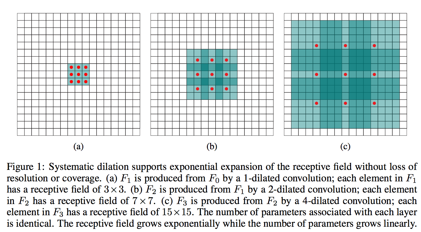
What this figure doesn't really show is the parameter sharing and parameter dependencies across the receptive field (frankly, it's pretty hard to visualise exactly with more than 2 layers). The receptive field grows at a faster rate than the number of parameters, and it is obvious that this can only be achieved by introducing additional constraints on the parameters across the receptive field. The network won't be able to learn arbitrary receptive field behaviours, so one question is, how severe is that restriction?
Relationship to Kronecker Products
To me this whole dilated convolution paper cries Kronecker product, although this connection is never made in the paper itself. It's easy to see that a 2D dilated convolution with matrix/filter $K$ is the same as vanilla convolution with a diluted filter $\hat{K}_{l}$ which can be represented as the following Kronecker product:
$$
\hat{K}_l = K \otimes
\begin{bmatrix}
1 & 0 & 0 & 0 & 0 \\
0 & 0 & \ddots & & 0 \\
0 & \ddots & \ddots & \ddots & \\
0 & & \ddots & \ddots & 0 \\
0 & 0 & 0 & 0 & 0
\end{bmatrix}
$$
Using this, and properties of convolutions and Kronecker products (I suggest beginners to make extensive use of the matrix cookbook) we can even understand something about exponentially iterated dilated convolutions.
Let's assume we apply several layers of dilated convolutions, without nonlinearity, as in Equation 3 of the paper. For simplicity, I assume that that all convolution kernels $K_l, L=1\ldots L$ are $a\times a$ in size, the dilation factor at layer $l$ is $a^{l}$, and we only have a single channel throughout ($C=1$). In this case we can show that:
$$
F_{L+1} = K_L \ast_{a^L} \left( K_{L-1} \ast_{a^{(L-1)}} \left( \cdots K_1 \ast_{a} \left( K_0 \ast F_0 \right) \cdots \right) \right) = \left( K_L \otimes K_{L-1} \otimes \cdots \otimes K_{0} \right) \ast F_0
$$
The left-hand side of this equation is the same construction as in Equation 3 in the paper, but expanded. The right hand side is a single vanilla convolution, but with a convolution kernel that is constructed as the Kronecker product of all the $a\times a$ kernels $K_l$.
It turns out Kronecker-factored parametrisations of convolution tensors are already used in CNNs, a quick googling revealed this paper:
- Shuchang Zhou, Jia-Nan Wu, Yuxin Wu, Xinyu Zhou (2015) Exploiting Local Structures with the Kronecker Layer in Convolutional Networks
What can Kronecker-factored filters represent?
Let's look at what kind of kernels can we represent with Kronecker products, and hence what behaviour should we expect from dilated convolutions. Here are a few examples of $27\times 27$ kernels that result from taking the Kronecker product of three random $3\times 3$ kernels:
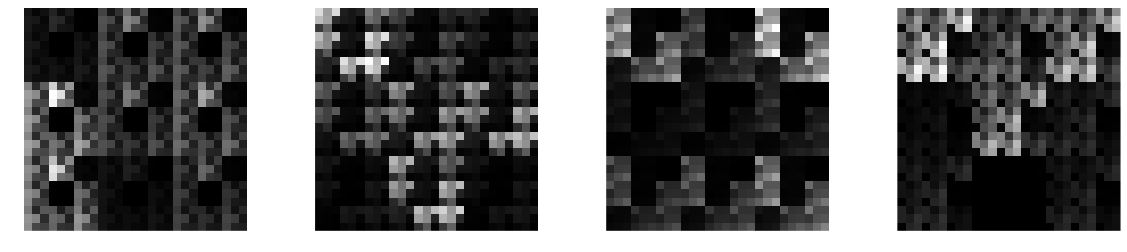
These look somehow natural, at least to me. They look like pretty plausible texture patches taken from some pixellated video game. You will notice the repeated patterns and the hierarchical structure. Indeed, we can draw cool self-similar fractal-like filters if we keep taking the Kronecker product of the same kernel with itself, some examples of such random fractals:
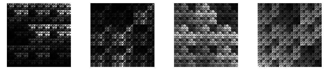
I would say these kernels are not entirely unreasonable for a ConvNet, and if you allow for multiple channels ($C>1$) they can represent pretty nice structured patterns and shapes with reasonable number of parameters.
Compare these filters to another common technique for reducing parameters of convolution tensors: low-rank decompositions (see e.g. Lebedev et al, 2014). Spatially, a low-rank approximation to a square 2D convolution filter can be understood as subsequently applying two smaller rectangular filters: one with a limited horizontal extent and one with limited vertical extent. Here are a few random samples of $27\times 27$ filters with a rank of 1. These can be represented using the same number of parameters (27) as the Kronecker samples above.
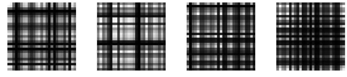
To me, these don't look so natural. Notice also that for low-rank representations the number of parameters has to scale linearly with the spatial extent of the filter, whereas this scaling can be logarithmic if we use a Kronecker parametrisation. This is the real deal when using Kronecker products or dilated convolutions.
Here is another cool illustration of the naturalness of the Kronecker approximation, taken out of the Kronecker layer paper:
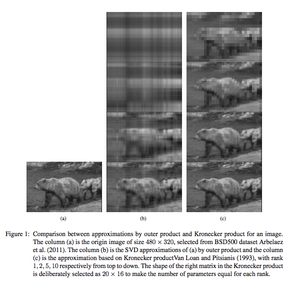
So in general, parametrising convolution kernels as Kronecker-products seems like a pretty good idea. The dilated convolutions paper presents a more flexible approach than just Kronecker-factors. Firstly, you can add nonlinearities after each layer of dilated convolution, which would now be different from Kronecker products. Secondly, the Kronecker analogy only holds if the dilation factor and the kernel size are the same. In the paper the authors used a kernel size of $3$ and dilation factor of $2$.
Final note on translational equivariance
One desirable property of convolutions is that they are translationally equivariant: if you shift the input image by any amount, the output remains the same, shifted by the same amount. This is a very useful inductive bias/prior assumtion to use in a dense prediction task.
One way to introduce multiscale thinking to ConvNets is to use architectures that look like the figure below: we first decrease the spatial extent of feature-maps via pooling, then grow them back again via unpooling/deconvolution. Additional shortcut connections ensure that pixel-level local accuracy can be retained. The example below is from the SegNet paper, but there are multiple other papers such as this one on recombinator networks.
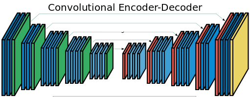
However, as soon as you include spatial pooling, the translational equivariance property of the whole network might break. For example the SegNet above is not translationally equivariant anymore: the network's predictions are sensitive to small, single-pixel shifts to the input image, which is undesirable. Thankfully, layers of dilated convolutions are still translationally equivariant, which is a good thing.
Summary
This dilated convolutions idea is pretty cool, and I think these papers are just scratching the surface of this topic. The dilated convolution architecture generalises Kronecker-factored convolutional filters, it allows for very large receptive fields while only growing the number of parameters logarithmically. [Zhou at al.] shows how you can use a similar idea in classification to achieve $3.6\times$ parameter reduction with only $1%$ drop of accuracy.
The composite kernels one obtains via Kronecker products look sensible and seem to have meaningful parameter-sharing assumptions (hierarchical organisation, self-similarity). Plus, the networks using only diluted convolutions are fully equivariant under translation, which is great for dense prediction applications.
On the negative side, CNNs have a problem at the edges of the image where the convolution needs to be padded. This often causes headaches in dense prediction. Dilated convolutions have an even bigger problem. I wonder how well these methods would do in applications like superresolution, particularly how well they would deal with borders of the image compared to the middle.